
Rを利用して固定効果モデルによる回帰を考えます。
以下の資料を引用参照しています。
- https://de.meta-analysis.com/download/Intro_Models.pdf
- https://pmc.ncbi.nlm.nih.gov/articles/PMC8924903/
- https://www.fbc.keio.ac.jp/~tyabu/econometrics/econome1_8.pdf
- https://www.nishiyama.kier.kyoto-u.ac.jp/2020/jugyochukei4.pdf
- https://user.keio.ac.jp/~nagakura/zemi/panel.pdf
以下の固定効果モデルを考えます。 \[Y_{i\,t} = \alpha_{i} + \beta X_{i\,t} + \epsilon_{i\,t} \tag{1}\] ここで、 \(Y_{i\,t}\) : 個体 i の時点 t における従属変数、\(\alpha_i\) : 個体 i の固定効果(個体ごとの切片)、\(X_{i\,t}\) : 個体 i の時点 t における説明変数、\(\beta\) : 説明変数の係数(すべての個体で共通)、\(\epsilon_{i\,t}\) : 誤差項
始めに固定効果と説明変数との間に相関のあるサンプルデータを作成します。
seed <- 20250126
set.seed(seed = seed)

n_id <- 5 # 個体数
n_time <- 6 # 時間数

# データフレームの作成
df <- data.frame(
  id = rep(1:n_id, each = n_time),
  time = rep(1:n_time, times = n_id)
)

# 個体効果(固定効果)を生成
id_effects <- rnorm(n_id, mean = 2, sd = 0.5)
df$id_effect <- id_effects[df$id]

# 固定効果と相関のある説明変数xを生成
df$x <- df$id_effect + rnorm(n_id * n_time, mean = 0, sd = 1) # id_effectに依存

# 誤差項を生成
df$epsilon <- rnorm(n_id * n_time, mean = 0, sd = 1)

# 従属変数yを生成
beta <- c(2, 3.5)
df$y <- beta[1] + beta[2] * df$x + df$id_effect + df$epsilon
サンプルデータを確認します。
library(dplyr)
library(ggplot2)
glimpse(df)
ggplot(data = df, mapping = aes(x = x, y = y, color = as.factor(id), shape = as.factor(id))) +
  geom_point(size = 2) +
  geom_smooth(method = "lm", se = F, linewidth = 0.1) +
  theme_minimal()
Rows: 30
Columns: 6
$ id <int> 1, 1, 1, 1, 1, 1, 2, 2, 2, 2, 2, 2, 3, 3, 3, 3, 3, 3, 4, 4, …
$ time <int> 1, 2, 3, 4, 5, 6, 1, 2, 3, 4, 5, 6, 1, 2, 3, 4, 5, 6, 1, 2, …
$ id_effect <dbl> 1.532956, 1.532956, 1.532956, 1.532956, 1.532956, 1.532956, …
$ x <dbl> 1.2236166, 0.5428839, -0.1687838, 1.9596749, 1.3257576, 2.52…
$ epsilon <dbl> 0.88224874, -1.35440156, -0.28777985, -0.12369397, -0.866977…
$ y <dbl> 8.697863, 4.078648, 2.654433, 10.268124, 7.306130, 11.229566…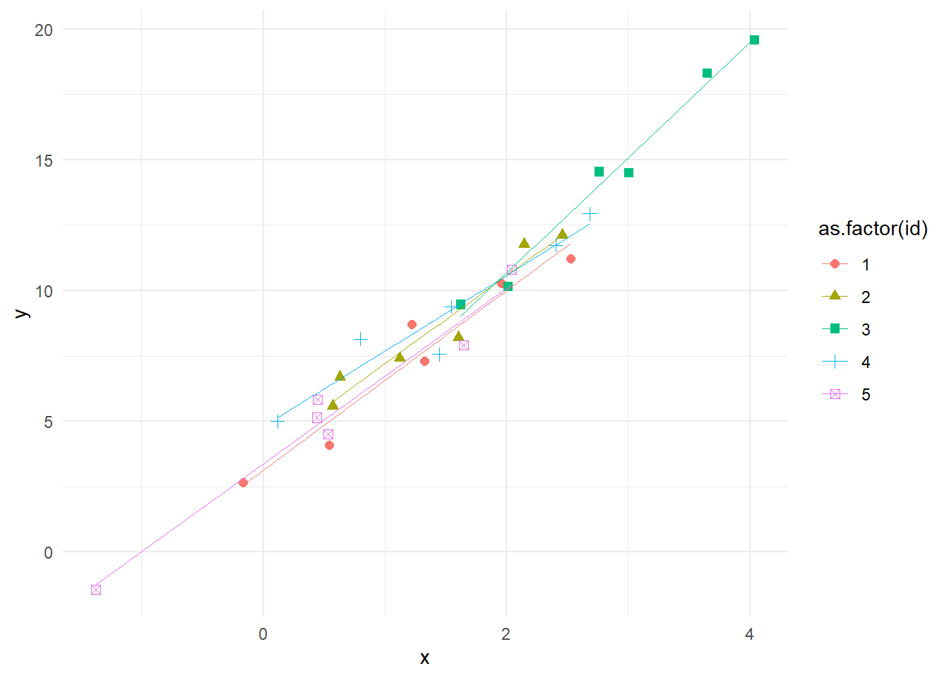
説明変数 x 固定効果 id_effect の相関を確認します。
cor(df$x, df$id_effect)[1] 0.6214152固定効果を考慮せずに線形回帰モデルを確認します。
lm(data = df, formula = y ~ x) %>% summary()
Call:
lm(formula = y ~ x, data = df)

Residuals:
    Min      1Q  Median      3Q     Max
-1.5614 -0.6340 -0.0320  0.7304  1.8422

Coefficients:
            Estimate Std. Error t value Pr(>|t|)
(Intercept)   3.3356     0.2781   11.99  1.5e-12 ***
x             3.7154     0.1455   25.53  < 2e-16 ***
---
Signif. codes:  0 '***' 0.001 '**' 0.01 '*' 0.05 '.' 0.1 ' ' 1

Residual standard error: 0.9177 on 28 degrees of freedom
Multiple R-squared:  0.9588,    Adjusted R-squared:  0.9573
F-statistic: 651.8 on 1 and 28 DF,  p-value: < 2.2e-16
固定効果を考慮した線形回帰モデルを確認します。
# 個体ごとの平均値を計算
df_means <- aggregate(. ~ id, data = df[, c("id", "y", "x")], FUN = mean)
names(df_means)[names(df_means) == "y"] <- "y_mean"
names(df_means)[names(df_means) == "x"] <- "x_mean"

df <- merge(df, df_means, by = "id")

# 各変数を平均値からの偏差に変換
df$y_demeaned <- df$y - df$y_mean
df$x_demeaned <- df$x - df$x_mean

# 偏差データを用いた線形回帰(最小二乗法)
X <- matrix(df$x_demeaned, ncol = 1)
Y <- matrix(df$y_demeaned, ncol = 1)

# 説明変数xの係数
beta_hat <- solve(t(X) %*% X) %*% t(X) %*% Y

# 残差の計算
residuals <- (Y - X %*% beta_hat) %>% as.vector()

# 残差平方和の計算
RSS <- sum(residuals^2)

# 自由度 (n - k)
k <- ncol(X)
n <- nrow(X)
degrees_of_freedom <- n - k - n_id

# 誤差分散の推定
sigma2_hat <- RSS / degrees_of_freedom

# 共分散行列の計算
var_beta_hat <- sigma2_hat * solve(t(X) %*% X)

# 標準誤差の計算
se_beta_hat <- sqrt(diag(var_beta_hat))

# 95%信頼区間の計算
alpha <- 0.05
critical_value <- qnorm(1 - alpha / 2) # 正規分布の臨界値

lower_ci <- beta_hat - critical_value * se_beta_hat # 下限
upper_ci <- beta_hat + critical_value * se_beta_hat # 上限

# 結果のまとめ
data.frame(beta_hat, var_beta_hat, se_beta_hat, lower_ci, upper_ci, check.names = F)
beta_hat var_beta_hat se_beta_hat lower_ci upper_ci
1 3.468962 0.0321274 0.1792412 3.117656 3.820268関数 plm{plm} を利用して固定効果モデルを求めます。
library(plm)
pdata <- pdata.frame(df[, c("id", "time", "x", "y")], index = c("id", "time"))
fixed_model <- plm(y ~ x, data = pdata, model = "within")
summary(fixed_model)
Oneway (individual) effect Within Model
Call:
plm(formula = y ~ x, data = pdata, model = "within")
Balanced Panel: n = 5, T = 6, N = 30
Residuals:
Min. 1st Qu. Median 3rd Qu. Max.
-1.374630 -0.595977 -0.023057 0.586923 1.444243
Coefficients:
Estimate Std. Error t-value Pr(>|t|)
x 3.46896 0.17924 19.354 3.77e-16 ***
---
Signif. codes: 0 '***' 0.001 '**' 0.01 '*' 0.05 '.' 0.1 ' ' 1
Total Sum of Squares: 304.44
Residual Sum of Squares: 18.332
R-Squared: 0.93978
Adj. R-Squared: 0.92724
F-statistic: 374.562 on 1 and 24 DF, p-value: 3.7698e-16分散共分散行列を確認します。
fixed_model$vcov x
x 0.032127495%信頼区間を確認します。
confint(fixed_model, level = .95) 2.5 % 97.5 %
x 3.117656 3.820268以上です。