
本ポスト作成に当たり以下の資料を引用参照しています。
- https://bkenkel.com/psci8357/notes/10-2sls.html
- https://ill-identified.hatenablog.com/entry/2015/01/07/233655
- https://www.ier.hit-u.ac.jp/~kitamura/lecture/Hit/08Statsys5.pdf
- https://user.keio.ac.jp/~nagakura/zemi/instrumental_variable.pdf
- https://www.fbc.keio.ac.jp/~tyabu/econometrics/econome1_13.pdf
- https://user.keio.ac.jp/~nagakura/R/R_2OLS.pdf
- https://user.keio.ac.jp/~nagakura/data/wagedata.txt
以下のモデルを考えます。
\[\begin{align} &\mathbf{y}=\boldsymbol{\beta}_0+\boldsymbol{\beta}_1\mathbf{x}_1+\boldsymbol{\beta}_2\mathbf{x}_2+\boldsymbol{\beta}_3\mathbf{x}_3+\boldsymbol{\epsilon}\\&\mathrm{cov}(\mathbf{x}_1,\boldsymbol{\epsilon})=\mathrm{cov}(\mathbf{x}_3,\boldsymbol{\epsilon})=0,\,\mathrm{cov}(\mathbf{x}_2,\boldsymbol{\epsilon})\neq0 \end{align} \tag{1}\] ここでは「説明変数のうち、\(\mathbf{x}_2\) のみが誤差項 \(\boldsymbol{\epsilon}\) と相関しているモデル」としています。
始めに説明変数 \(\mathbf{x}_2\) と 誤差項 \(\boldsymbol{\epsilon}\) との相関を考慮せずに最小二乗法のシミュレーション結果を確認します。
以下のコードで最小二乗法で求めた係数を取り出します。
なお、操作変数の一つとする \(\mathrm{z}\) は \(\boldsymbol{\epsilon}\) および他の説明変数とは相関せず、\(\mathrm{x}_2\) とのみ相関している変数です。サンプルですので操作変数を最初から準備してしまいます。
library(dplyr)
fun_simulate_ls <- function(iter = 1000, n = 1000, beta) {
  for (i in seq(iter)) {
    set.seed(i)
    # サンプルデータの作成
    ## 外生変数
    x1 <- rnorm(n)
    x3 <- rnorm(n)
    ## 操作変数。
    z <- rnorm(n)
    ## 誤差項
    e <- rnorm(n)
    ## 内生変数
    x2 <- z + e
    ## 従属変数
    beta <- beta %>% matrix(ncol = 1)
    X <- data.frame(1, x1, x2, x3) %>% as.matrix()
    y <- X %*% beta + e
    # 内生性を考慮しない最小二乗法
    ls_coef <- lm(y ~ x1 + x2 + x3)$coef %>%
      t() %>%
      data.frame(check.names = F)
    if (i == 1) {
      result_ls <- ls_coef
    } else {
      result_ls <- rbind(result_ls, ls_coef)
    }
  }
  return(result_ls)
}
result_ls <- fun_simulate_ls(iter = 1000, n = 1000, beta = c(2, 3, 4, -2))
result_ls %>% glimpse()
Rows: 1,000
Columns: 4
$ `(Intercept)` <dbl> 2.000365, 1.981592, 2.002458, 1.993495, 1.988178, 1.9873…
$ x1 <dbl> 2.986904, 2.967904, 2.977572, 3.046114, 3.012441, 3.0514…
$ x2 <dbl> 4.504145, 4.484650, 4.502343, 4.499104, 4.476267, 4.5005…
$ x3 <dbl> -2.003480, -1.973751, -1.975065, -2.010949, -1.981412, -…ヒストグラムでシミュレーション結果を確認します。
library(ggplot2)
result_ls %>%
  tidyr::gather(value = "Estimate") %>%
  ggplot(mapping = aes(x = Estimate)) +
  geom_histogram(binwidth = 0.01, position = "identity", color = "white") +
  facet_wrap(. ~ key, scales = "free") +
  theme_minimal()
シミュレーションでは \(\mathbf{x}_2\) の係数を「4」 と設定しましたが、Figure 1 の左下のヒストグラムのとおり、影響が「過大評価」されています。
\(\mathbf{x}_2\) の係数を「-1」 としてもう一度。
result_ls <- fun_simulate_ls(iter = 1000, n = 1000, beta = c(2, 3, -1, -2))
result_ls %>%
  tidyr::gather(value = "Estimate") %>%
  ggplot(mapping = aes(x = Estimate)) +
  geom_histogram(binwidth = 0.01, position = "identity", color = "white") +
  facet_wrap(. ~ key, scales = "free") +
  theme_minimal()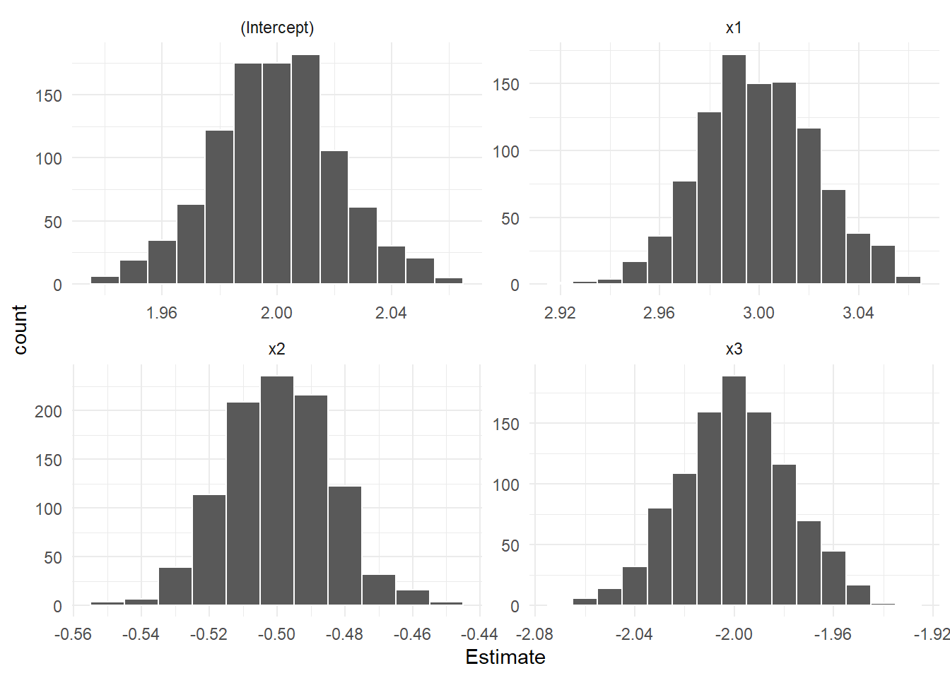
同様に \(\mathbf{x}_2\) の影響が正の方向に「過大評価」されています。
続いて2段階最小二乗法によるシミュレーション結果を確認します。
第1段階では操作変数を含む外生変数 \(\mathbf{x}_1,\mathbf{x}_3,\mathbf{z}\) で \(\mathbf{x}_2\) を回帰することにより、\(\mathbf{x}_2\) から外生変数によって説明される部分(誤差項と相関しない部分)を抽出します。
よって、外生変数と相関する部分が誤差項の一部として残ることは無くなりますので、\(\hat{\mathbf{x}}_2\) と誤差項 \(\boldsymbol{\epsilon}\) との相関は消失します。
第1段階で求めた \(\hat{\mathbf{x}}_2\) は \(\boldsymbol{\epsilon}\) とは相関していませんので、第2段階における説明変数はいずれも \(\boldsymbol{\epsilon}\) と相関していないことになります。
fun_simulate_tsls <- function(iter = 1000, n = 1000, beta) {
  for (i in seq(iter)) {
    set.seed(i)
    # サンプルデータ作成パート
    ## 外生変数
    x1 <- rnorm(n)
    x3 <- rnorm(n)
    ## 操作変数
    z <- rnorm(n)
    ## 誤差項
    e <- rnorm(n)
    ## 内生変数
    x2 <- z + e
    ## 従属変数
    beta <- beta %>% matrix(ncol = 1)
    X <- data.frame(1, x1, x2, x3) %>% as.matrix()
    y <- X %*% beta + e
    # 2段階最小二乗法
    ## 第1段階 : 内生変数を操作変数で回帰
    stage1 <- lm(x2 ~ x1 + x3 + z)
    ### 内生変数の予測値を計算
    x2_hat <- predict(stage1)
    ## 第2段階: 従属変数を予測された内生変数と外生変数で回帰
    stage2 <- lm(y ~ x1 + x2_hat + x3)
    # 係数の取得
    tsls_coef <- stage2$coef %>%
      t() %>%
      data.frame(check.names = F)
    if (i == 1) {
      result_tsls <- tsls_coef
    } else {
      result_tsls <- rbind(result_tsls, tsls_coef)
    }
  }
  return(result_tsls)
}
result_tsls <- fun_simulate_tsls(iter = 1000, n = 1000, beta = c(2, 3, 4, -2))
result_tsls %>% glimpse()
Rows: 1,000
Columns: 4
$ `(Intercept)` <dbl> 2.016938, 2.022837, 1.992243, 2.000968, 1.977521, 2.0103…
$ x1 <dbl> 3.022791, 2.939377, 2.970326, 3.069847, 3.025095, 3.0399…
$ x2_hat <dbl> 4.009185, 4.041071, 4.052703, 3.979075, 4.019005, 3.9887…
$ x3 <dbl> -1.984976, -1.953947, -1.986519, -1.969224, -1.974155, -…result_tsls %>%
tidyr::gather(value = "Estimate") %>%
ggplot(mapping = aes(x = Estimate)) +
geom_histogram(binwidth = 0.01, position = "identity", color = "white") +
facet_wrap(. ~ key, scales = "free") +
theme_minimal()
\(\mathbf{x}_2\) の係数を「-1」 としてもう一度。
result_tsls <- fun_simulate_tsls(iter = 1000, n = 1000, beta = c(2, 3, -1, -2))
result_tsls %>%
  tidyr::gather(value = "Estimate") %>%
  ggplot(mapping = aes(x = Estimate)) +
  geom_histogram(binwidth = 0.01, position = "identity", color = "white") +
  facet_wrap(. ~ key, scales = "free") +
  theme_minimal()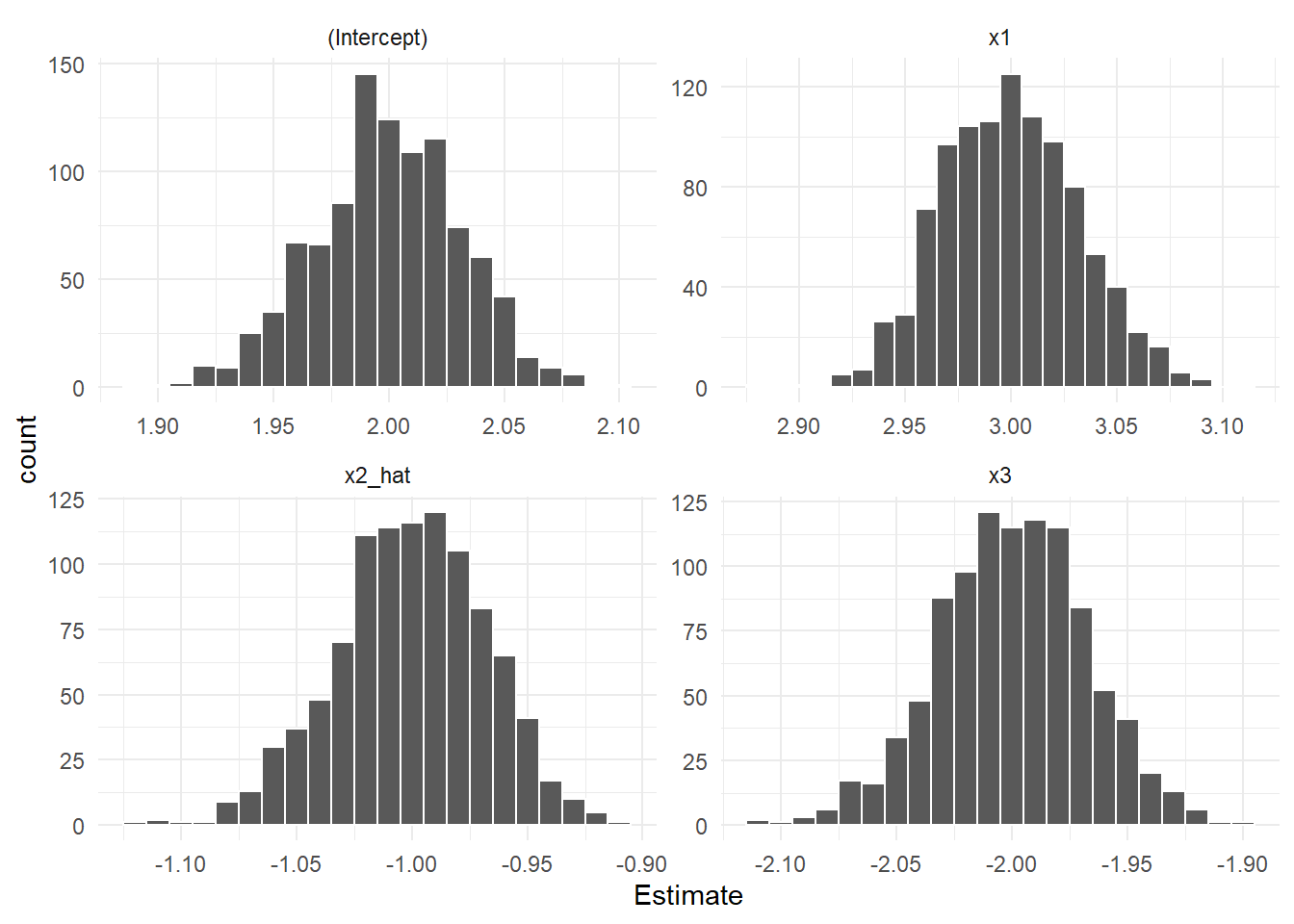
「内生変数(ここでは \(\mathbf{x}_2\))とは相関しているが他の説明変数および誤差項とは相関していない変数(操作変数)」を利用すれば、バイアスのないパラメータを求めることが確認できました。
「内生変数とは相関しているが他の説明変数および誤差項とは相関していない変数」。。。「言うは易く行うは難し」ですね。
Rでは 関数 ivreg {AER} と tsls {sem} を利用して2段階最小二乗法を行えます。
始めにサンプルデータを作成します。
set.seed(20250106)
beta <- c(-2, 3, -1, 4)
n <- 1000
x1 <- rnorm(n)
x3 <- rnorm(n)
z <- rnorm(n)
e <- rnorm(n)
x2 <- z + e
beta <- beta %>% matrix(ncol = 1)
X <- data.frame(1, x1, x2, x3) %>% as.matrix()
y <- X %*% beta + e
stage1 <- lm(x2 ~ x1 + x3 + z)
x2_hat <- predict(stage1)
(stage2 <- lm(y ~ x1 + x2_hat + x3))
Call:
lm(formula = y ~ x1 + x2_hat + x3)

Coefficients:
(Intercept)           x1       x2_hat           x3
     -2.011        2.995       -0.992        3.998
関数 ivreg {AER} によります。
AER::ivreg(formula = y ~ x1 + x2 + x3 | x1 + z + x3)
Call:
AER::ivreg(formula = y ~ x1 + x2 + x3 | x1 + z + x3)

Coefficients:
(Intercept)           x1           x2           x3
     -2.011        2.995       -0.992        3.998
関数 tsls {sem} によります。
sem::tsls(formula = y ~ x1 + x2 + x3, instruments = ~ x1 + z + x3)
Model Formula: y ~ x1 + x2 + x3

Instruments: ~x1 + z + x3

Coefficients:
(Intercept)          x1          x2          x3
 -2.0107172   2.9950812  -0.9920422   3.9980926
以上です。