
Rによる 完全実施要因計画 を試みます。
ここでは、2つの因子(AとB)があり、それぞれが2つの水準を持つ、22要因計画(2の2乗要因計画)をシミュレーションします。
シミュレーションのシナリオは以下の通りです。
- 因子A : 温度(水準: “低温”, “高温”)
- 因子B : 圧力(水準: “低圧”, “高圧”)
- 応答Y : 製品の収率(数値)
- 仮定する真の効果 :
- 温度が高いと収率が上がる(主効果A)
- 圧力が高いと収率が上がる(主効果B)
- 温度と圧力が両方高い場合に、相乗効果でさらに収率が上がる(交互作用AB)
- 実験の繰り返し : 各条件で3回実験を繰り返す
パッケージの読み込みと乱数seedを設定します。
library(dplyr)
library(ggplot2)
seed <- 20250510
1. 因子と水準の設定
factor_A_levels <- factor(c("低温", "高温"), levels = c("低温", "高温"))
factor_B_levels <- factor(c("低圧", "高圧"), levels = c("低圧", "高圧"))
# factor_A_levels <- factor(c("低温", "高温"))
# factor_A_levels <- relevel(factor_A_levels,"低温")
# factor_B_levels <- factor(c("低圧", "高圧"))
# factor_B_levels <- relevel(factor_B_levels,"低圧")
2. 完全実施要因計画の生成
# 計画行列(デザインマトリックス)の作成
doe_plan_unique <- expand.grid(
  A = factor_A_levels,
  B = factor_B_levels
)

print("基本的な実験計画 (各条件1回):")
print(doe_plan_unique)
[1] "基本的な実験計画 (各条件1回):"
A B
1 低温 低圧
2 高温 低圧
3 低温 高圧
4 高温 高圧# 各実験条件での繰り返し回数
n_replicates <- 3
# 繰り返しを考慮した実験計画を作成
# 各行をn_replicates回繰り返す
doe_plan_replicated <- doe_plan_unique[rep(seq_len(nrow(doe_plan_unique)), each = n_replicates), ]
rownames(doe_plan_replicated) <- NULL # 行名をリセット
print(paste("繰り返しを含む実験計画 (各条件", n_replicates, "回):"))
print(doe_plan_replicated)[1] "繰り返しを含む実験計画 (各条件 3 回):"
A B
1 低温 低圧
2 低温 低圧
3 低温 低圧
4 高温 低圧
5 高温 低圧
6 高温 低圧
7 低温 高圧
8 低温 高圧
9 低温 高圧
10 高温 高圧
11 高温 高圧
12 高温 高圧3. 応答変数の生成(シミュレーション)
# 応答Y(製品の収率)をシミュレートします。
# 真のモデルを以下のように仮定します:
# Y = 切片 + Aの効果 + Bの効果 + AB交互作用効果 + 誤差

# 真のパラメータを設定
intercept_true <- 60 # ベースラインの収率
effect_A_high_true <- 15 # Aが"高温"であることによる収率増
effect_B_high_true <- 10 # Bが"高圧"であることによる収率増
effect_AB_interaction_true <- 8 # Aが"高温"かつBが"高圧"であることによる追加の収率増 (交互作用)
error_sd_true <- 2.5 # 実験誤差の標準偏差

# 乱数のシードを設定
set.seed(seed)

# 応答Yを計算する関数
generate_response <- function(A_level, B_level) {
  y <- intercept_true
  if (A_level == "高温") {
    y <- y + effect_A_high_true
  }
  if (B_level == "高圧") {
    y <- y + effect_B_high_true
  }
  if (A_level == "高温" && B_level == "高圧") {
    y <- y + effect_AB_interaction_true
  }
  # 正規分布に従う誤差を加える
  y <- y + rnorm(1, mean = 0, sd = error_sd_true)
  return(y)
}

# 各実験条件に対して応答Yを生成
sim_data <- doe_plan_replicated %>%
  mutate(Y = mapply(generate_response, A, B))

print("シミュレーションデータ (応答Yを含む):")
print(sim_data)
[1] "シミュレーションデータ (応答Yを含む):"
A B Y
1 低温 低圧 59.34116
2 低温 低圧 61.92632
3 低温 低圧 65.11543
4 高温 低圧 75.22094
5 高温 低圧 73.45216
6 高温 低圧 69.99049
7 低温 高圧 73.49652
8 低温 高圧 71.01753
9 低温 高圧 69.25795
10 高温 高圧 94.56928
11 高温 高圧 90.93631
12 高温 高圧 95.345174. データの分析 (線形モデルの当てはめ)
# 因子A、因子B、およびそれらの交互作用A:Bをモデルに含めます。
# A*B は A + B + A:B と同じ。
model <- lm(Y ~ A * B, data = sim_data)

# 分析結果のサマリーを表示
print("モデルのサマリー (summary):")
summary(model)
[1] "モデルのサマリー (summary):"
Call:
lm(formula = Y ~ A * B, data = sim_data)
Residuals:
Min 1Q Median 3Q Max
-2.8974 -2.1697 0.1815 1.8560 2.9878
Coefficients:
Estimate Std. Error t value Pr(>|t|)
(Intercept) 62.128 1.458 42.604 1.02e-10 ***
A高温 10.760 2.062 5.218 0.000805 ***
B高圧 9.130 2.062 4.427 0.002206 **
A高温:B高圧 11.599 2.917 3.977 0.004078 **
---
Signif. codes: 0 '***' 0.001 '**' 0.01 '*' 0.05 '.' 0.1 ' ' 1
Residual standard error: 2.526 on 8 degrees of freedom
Multiple R-squared: 0.9689, Adjusted R-squared: 0.9573
F-statistic: 83.2 on 3 and 8 DF, p-value: 2.261e-06# 推定係数の95%信頼区間を表示
print("推定係数の95%信頼区間:")
confint(object = model, level = 0.95)[1] "推定係数の95%信頼区間:"
2.5 % 97.5 %
(Intercept) 58.764873 65.49040
A高温 6.004560 15.51589
B高圧 4.374027 13.88536
A高温:B高圧 4.873837 18.324895. 結果の解釈とポイント
- summary(model) の見方:
- Coefficients:
- Estimate: 各項の係数の推定値。
- (Intercept): A=“低温”, B=“低圧” (基準水準)のときのYの平均値の推定。
- A高温:Aが”低温”から”高温”に変わったときのYの変化量の推定 (Bが”低圧”のとき)。
- B高圧:Bが”低圧”から”高圧”に変わったときのYの変化量の推定 (Aが”低温”のとき)。
- A高温:B高圧: 交互作用効果の推定。Aが”高温”であり、かつBが”高圧”である場合に、それぞれの主効果だけでは説明できない追加の効果。
- Std. Error: 係数の標準誤差。
- t value: t統計量 (Estimate / Std. Error)。
- Pr(>|t|): p値。
- Estimate: 各項の係数の推定値。
- Coefficients:
- 今回のシミュレーションでは、A、B、A:Bの全ての効果を意図的に入れているため、効果が有意(5%)であると検出されています。
6. 結果の可視化
始めに 因子Aの主効果をプロット。
main_effect_A_plot <- sim_data %>%
  group_by(A) %>%
  summarise(mean_Y = mean(Y), .groups = "drop") %>%
  ggplot(aes(x = A, y = mean_Y, group = 1)) +
  geom_line(linewidth = 1) +
  geom_point(size = 3) +
  labs(title = "因子Aの主効果プロット", x = "因子A (温度)", y = "平均収率 Y") +
  ylim(min(sim_data$Y) - 5, max(sim_data$Y) + 5) +
  theme_minimal()
print(main_effect_A_plot)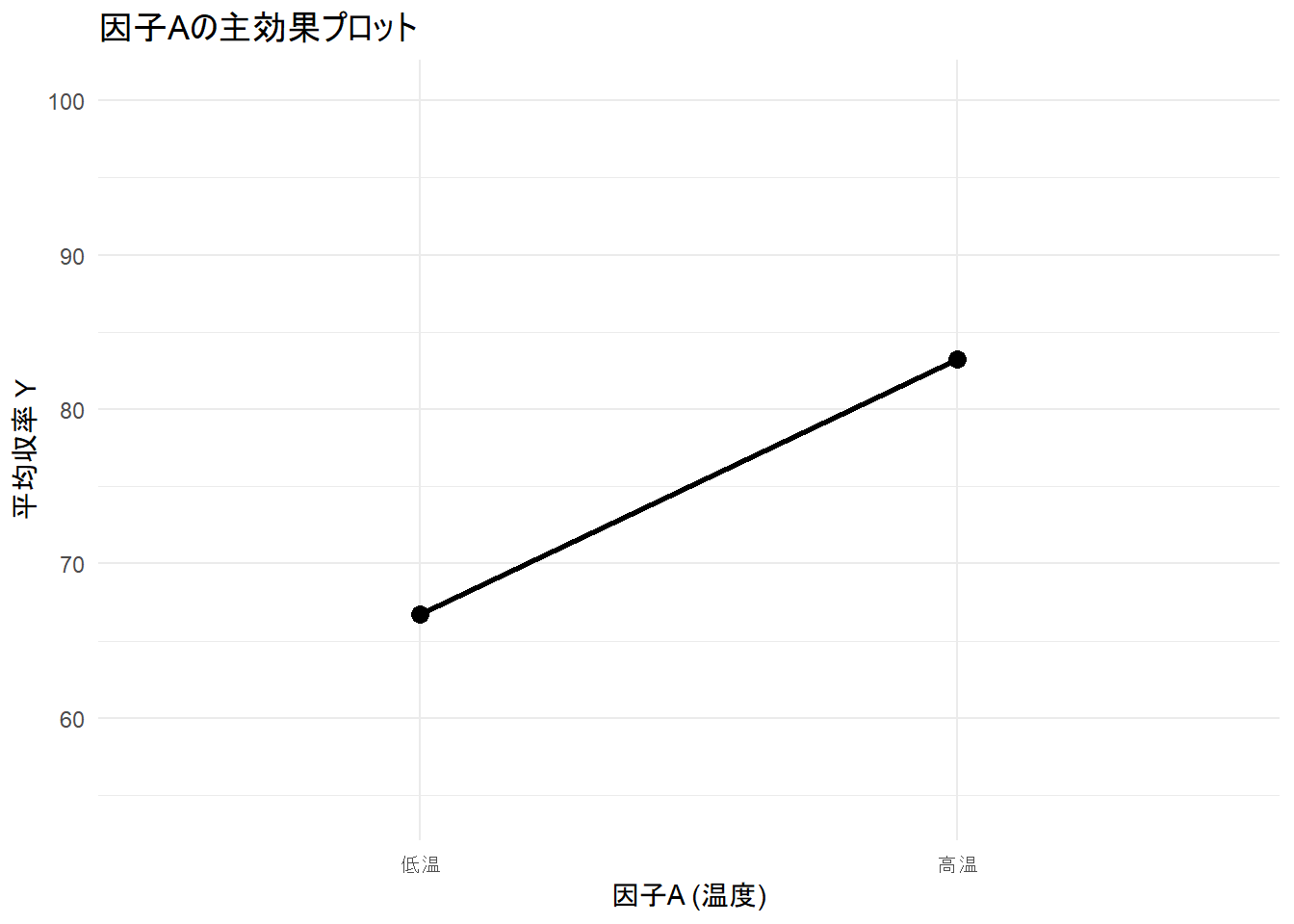
続いて 因子Bの主効果をプロット。
main_effect_B_plot <- sim_data %>%
  group_by(B) %>%
  summarise(mean_Y = mean(Y), .groups = "drop") %>%
  ggplot(aes(x = B, y = mean_Y, group = 1)) +
  geom_line(linewidth = 1) +
  geom_point(size = 3) +
  labs(title = "因子Bの主効果プロット", x = "因子B (圧力)", y = "平均収率 Y") +
  ylim(min(sim_data$Y) - 5, max(sim_data$Y) + 5) +
  theme_minimal()
print(main_effect_B_plot)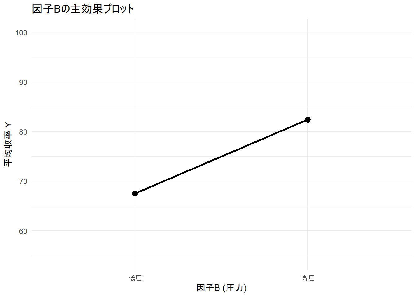
最後は 交互作用をプロット。
interaction_plot_gg <- sim_data %>%
  group_by(A, B) %>%
  summarise(mean_Y = mean(Y), .groups = "drop") %>%
  ggplot(aes(x = A, y = mean_Y, group = B, color = B, shape = B)) +
  geom_line(linewidth = 1) +
  geom_point(size = 4) +
  labs(
    title = "交互作用プロット (温度 vs 圧力)",
    x = "因子A (温度)",
    y = "平均収率 Y",
    color = "因子B (圧力)",
    shape = "因子B (圧力)"
  ) +
  ylim(min(sim_data$Y) - 5, max(sim_data$Y) + 5) +
  theme_minimal()
print(interaction_plot_gg)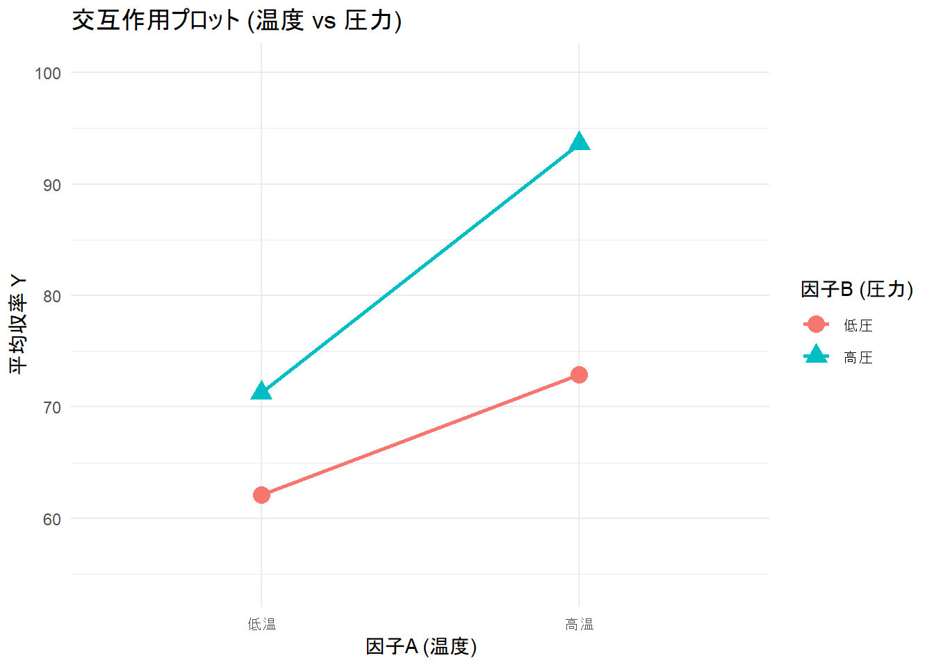
- 線が平行であれば、交互作用は小さいか、存在しないことを示唆します。
- 線が平行でない(交差したり、一方の因子のある水準で線の間隔が他と異なるなど)場合、 交互作用が存在することを示唆します。
- 今回のシミュレーションでは、A=“高温”かつB=“高圧”のときに特にYが大きくなるように設定しましたので、 交互作用プロットで線が平行でなく、「高温」の点で「低圧」の線と「高圧」の線の差が、「低温」の点での差よりも大きくなっています(上に開いています)。
以上です。