Rの関数:VAR {vars} 引数 exogen の利用

Rの関数から VAR {vars} 引数 exogen の利用 を確認します。

本ポストはこちらの続きです。

Rの関数から VAR {vars} 引数 season の利用を確認します。本ポストはこちらの続きです。シミュレーションの設計データの構造:四半期データ（1年＝4期）を想定し、season = 4 を設定します。季節性の導入:変数A (S...

シミュレーションの設計

データの構造:
- 内生変数 (y_1, y_2): 互いに影響し合う2つの変数（VAR構造）。
- 外生変数 (x): システムの外側から y_1, y_2 に「衝撃（ショック）」を与える変数。y は x に影響を与えません。
係数の設定:
- VAR係数 (内生): 以前と同様のラグ構造を設定します。
- 外生係数:
  - x が y_1 に与える影響: +2.0
  - x が y_2 に与える影響: -1.5
目的:
- exogen 引数を使ってモデルを推定した際に、VARのラグ係数だけでなく、「外部からの衝撃の効果（+2.0 と -1.5）」を正しく分離して推定できるかを確認します。

なお、有意水準は5%とします。

Rコード

外生変数 (exogen) を含むVARデータの生成

観測数: 200
内生変数: Endo_A, Endo_B (相互に影響)
外生変数: Exogen_X (外部から Endo_A, Endo_B に影響を与える)
真の外生係数: Endo_Aへの影響 = +2.0, Endo_Bへの影響 = -1.5

# パッケージの読み込み
library(vars)
library(ggplot2)
library(tidyr)

# 乱数シードの固定
seed <- 20260103
set.seed(seed)

# 設定: 2変量VAR(1) + 1変量外生変数
n_obs <- 200

# 1. VARの真の係数 (内生変数のラグ効果)
# y1(t) = 0.5 * y1(t-1) + 0.2 * y2(t-1) ...
# y2(t) = -0.3 * y1(t-1) + 0.4 * y2(t-1) ...
A_true <- matrix(c(0.5, 0.2, -0.3, 0.4), nrow = 2, byrow = TRUE)

# 2. 外生変数の係数 (Impact of Exogenous Variable)
# x(t) が現在の y1, y2 に与える影響
# y1 に対して: +2.0
# y2 に対して: -1.5
B_exogen <- matrix(c(2.0, -1.5), nrow = 2)

# 外生変数 x の生成 (ランダムな外部ショック)
# 正規乱数で生成
x_t <- rnorm(n_obs, mean = 0, sd = 1)

# データ生成
data_y <- matrix(0, nrow = n_obs, ncol = 2)
colnames(data_y) <- c("Endo_A", "Endo_B")

# 初期値
y_prev <- matrix(c(0, 0), ncol = 1)

for (t in 2:n_obs) {
  # 外生変数の値 (現在の時点 t の値を使用)
  x_curr <- x_t[t]

  # y(t) = A * y(t-1) + B * x(t) + error
  # ここで x(t) が加算される点が重要です
  y_curr <- A_true %*% y_prev + B_exogen * x_curr + rnorm(2, sd = 0.5)

  data_y[t, ] <- as.vector(y_curr)
  y_prev <- y_curr
}

# データフレーム化
df_sim <- as.data.frame(data_y)
df_sim$Exogen_X <- x_t
df_sim$Time <- 1:n_obs

# データの可視化
# 外生変数Xと、内生変数Endo_Aの動きを比較
p1 <- ggplot(df_sim, aes(x = Time)) +
  geom_line(aes(y = Endo_A, color = "内生変数 Endo_A"), alpha = 0.8) +
  geom_line(aes(y = Exogen_X, color = "外生変数 X"), alpha = 0.6, linetype = "dashed") +
  labs(
    title = "外生変数と内生変数の推移",
    subtitle = "外生変数X（点線）の動きに呼応して、Endo_A（実線）が変動している様子",
    x = "時間", y = "値"
  ) +
  scale_color_manual(name = "変数", values = c("内生変数 Endo_A" = "blue", "外生変数 X" = "red")) +
  theme_minimal()

print(p1)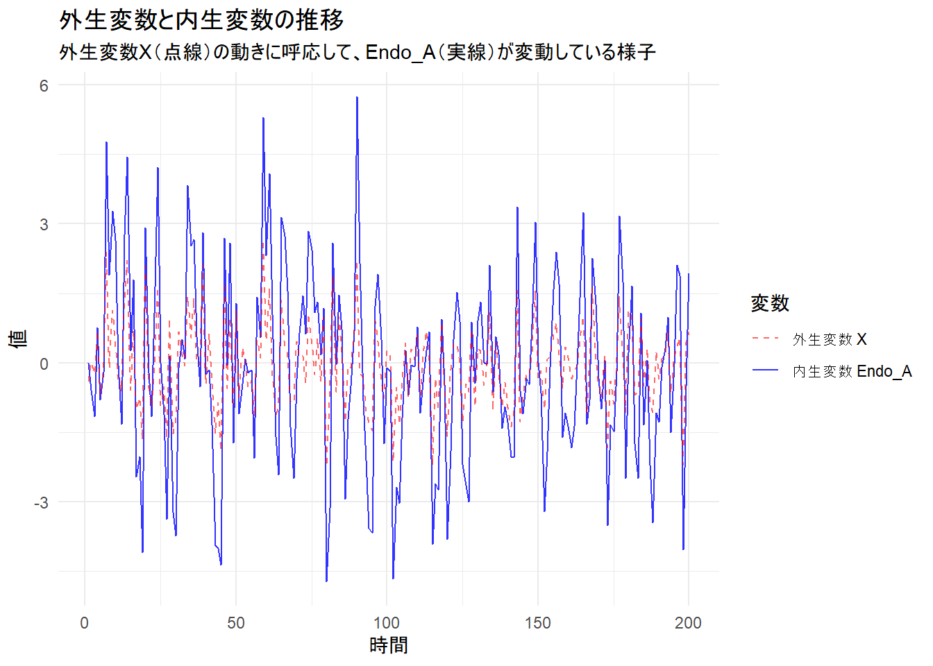

VARモデルの推定 (exogen引数の利用)

# 推定の実行
# y引数には内生変数のみを渡す
# exogen引数に外生変数を渡す
# exogenの行数は y と同じである必要があります

exogen_data <- matrix(df_sim$Exogen_X, ncol = 1)
colnames(exogen_data) <- "Exo_X"

var_exogen <- VAR(
  y = df_sim[, c("Endo_A", "Endo_B")],
  p = 1,
  type = "const",
  exogen = exogen_data
)

print(summary(var_exogen))


VAR Estimation Results:
========================= 
Endogenous variables: Endo_A, Endo_B 
Deterministic variables: const 
Sample size: 199 
Log Likelihood: -279.56 
Roots of the characteristic polynomial:
0.5578 0.5578
Call:
VAR(y = df_sim[, c("Endo_A", "Endo_B")], p = 1, type = "const", 
    exogen = exogen_data)


Estimation results for equation Endo_A: 
======================================= 
Endo_A = Endo_A.l1 + Endo_B.l1 + const + Exo_X 

           Estimate Std. Error t value Pr(>|t|)    
Endo_A.l1  0.547005   0.028013  19.527  < 2e-16 ***
Endo_B.l1  0.262998   0.029923   8.789 7.83e-16 ***
const     -0.002462   0.035989  -0.068    0.946    
Exo_X      1.958758   0.038473  50.913  < 2e-16 ***
---
Signif. codes:  0 '***' 0.001 '**' 0.01 '*' 0.05 '.' 0.1 ' ' 1


Residual standard error: 0.5027 on 195 degrees of freedom
Multiple R-Squared: 0.9419, Adjusted R-squared: 0.941 
F-statistic:  1053 on 3 and 195 DF,  p-value: < 2.2e-16 


Estimation results for equation Endo_B: 
======================================= 
Endo_B = Endo_A.l1 + Endo_B.l1 + const + Exo_X 

          Estimate Std. Error t value Pr(>|t|)    
Endo_A.l1 -0.31016    0.02699 -11.494   <2e-16 ***
Endo_B.l1  0.41958    0.02883  14.556   <2e-16 ***
const      0.01328    0.03467   0.383    0.702    
Exo_X     -1.49642    0.03706 -40.377   <2e-16 ***
---
Signif. codes:  0 '***' 0.001 '**' 0.01 '*' 0.05 '.' 0.1 ' ' 1


Residual standard error: 0.4843 on 195 degrees of freedom
Multiple R-Squared: 0.9388, Adjusted R-squared: 0.9378 
F-statistic: 996.6 on 3 and 195 DF,  p-value: < 2.2e-16 



Covariance matrix of residuals:
          Endo_A    Endo_B
Endo_A 0.2527439 0.0001642
Endo_B 0.0001642 0.2345434

Correlation matrix of residuals:
          Endo_A    Endo_B
Endo_A 1.0000000 0.0006746
Endo_B 0.0006746 1.0000000

Endo_A の方程式：外部からのプラスの衝撃

シミュレーション設定（真の値）:

ラグ効果:
- 自身の過去(0.5)、相手の過去(0.2)
外生効果:
- 外部ショックXから +2.0 の影響

結果の解釈

Endo_A.l1 (0.547) & Endo_B.l1 (0.263):
- 真の値 (0.5 と 0.2) に近い値が推定されています。自己回帰の構造が正しく捉えられています。
Exo_X (1.959):
- 真の値 2.0 に近い値が推定され、p値は設定した有意水準を下回っています。「外部要因Xが1単位増えると、Endo_Aは2単位増える」という関係性を特定できています。

Endo_B の方程式：外部からのマイナスの衝撃

シミュレーション設定（真の値）:

ラグ効果:
- 相手の過去(-0.3)、自身の過去(0.4)
外生効果:
- 外部ショックXから -1.5 の影響

結果の解釈

Endo_A.l1 (-0.310) & Endo_B.l1 (0.420):
- こちらも真の値 (-0.3 と 0.4) に近い値となっています。
Exo_X (-1.496):
- 真の値 -1.5 とほぼ一致しており、p値は設定した有意水準を下回っています。「外部要因Xが増えると、Endo_Bは減少する」という逆方向の因果関係も特定できています。

モデル全体の評価

決定係数 (Multiple R-Squared):
- 両方程式ともに 約0.94 と高い値を示しています。これは、内生変数の変動のほとんどが、「過去の履歴」と「現在の外部ショック」によって説明できていることを意味します。
残差の相関 (Correlation matrix of residuals):
- Endo_A と Endo_B の残差間の相関は 0.00067 とほぼゼロです。モデルが構造（ラグと外生要因）を適切に吸い上げたため、残った誤差には何の関係性も残っていない状態です。

以上です。