
RStan を利用して MCMCにおけるパラメーター非中心化の効果 を確認します。
ステップ1:サンプルデータの作成
まず、Rでシミュレーションデータを作成します。
- 意図的に グループ間のばらつきが小さく、各グループのデータが少ない 階層モデルをサンプルとします。
- 20個のグループ (
J=20) - 各グループに3つのデータ点 (
N_per_group=3) - グループ間のばらつき (
sigma_theta) を意図的に小さく設定 (0.5)
この設定により、非中心化しないモデルでは「Divergent Transitions」が発生しやすくなると考えられます。
# RStanの読み込み
library(rstan)

stan_output <- "D:/stan_output"

# Stanの並列計算設定
rstan_options(auto_write = TRUE)
options(mc.cores = parallel::detectCores())

# rstan のバージョン確認
cat("--- パッケージ rstan のバージョン確認 ---\n")
sapply(X = c("rstan"), packageVersion)
--- パッケージ rstan のバージョン確認 ---
$rstan
[1] 2 32 7# 1. サンプルデータの生成
# ------------------------------------
seed <- 20250629
set.seed(seed)
J <- 20 # グループ数
N_per_group <- 3 # 各グループのデータ数
N <- J * N_per_group # 全データ数
mu_theta_true <- 5 # グループ平均の全体平均
sigma_theta_true <- 0.5 # グループ平均のばらつき(小さく設定)
sigma_y_true <- 2 # 観測誤差の標準偏差
# グループごとの真の平均 theta を生成
theta_true <- rnorm(J, mean = mu_theta_true, sd = sigma_theta_true)
# 観測データ y を生成
y <- c()
group_id <- c()
for (j in 1:J) {
y <- c(y, rnorm(N_per_group, mean = theta_true[j], sd = sigma_y_true))
group_id <- c(group_id, rep(j, N_per_group))
}
# Stanに渡すためのデータリスト
stan_data <- list(
N = N,
J = J,
y = y,
group_id = group_id
)
cat("--- Stanに渡すデータの確認 ---\n")
stan_data--- Stanに渡すデータの確認 ---
$N
[1] 60
$J
[1] 20
$y
[1] 5.3924234 4.4354016 3.9094285 8.1098320 5.1711431 3.1792661
[7] 2.0543359 4.0288667 7.4404240 2.9698163 5.7729112 5.2764629
[13] 3.9012393 3.2080973 5.6239613 3.1773727 5.0124879 4.6049246
[19] 8.4291529 6.8349197 3.4123091 7.4894056 4.0500269 1.1571312
[25] 5.6930797 4.0882532 5.5924185 4.3354823 6.0164813 5.9066664
[31] 5.1354331 5.7345194 5.4324633 7.9379117 4.7057127 2.7067251
[37] -0.0947001 1.5147723 5.3050856 6.1310973 6.1882418 4.1333137
[43] 5.4043420 2.3422923 4.6041155 2.7290008 4.7206715 8.7479012
[49] 5.2370215 3.1579747 4.1220437 9.3209726 4.1703008 5.5390429
[55] 6.3114662 5.2919338 6.0616842 4.2912314 8.1858573 7.4744017
$group_id
[1] 1 1 1 2 2 2 3 3 3 4 4 4 5 5 5 6 6 6 7 7 7 8 8 8 9
[26] 9 9 10 10 10 11 11 11 12 12 12 13 13 13 14 14 14 15 15 15 16 16 16 17 17
[51] 17 18 18 18 19 19 19 20 20 20ステップ2:Stanコードの作成
次に、2種類のStanコードを作成します。
a. 非中心化しないモデル
パラメータthetaがmu_thetaとsigma_thetaに直接依存する、直感的な書き方です。
model_code <- "
data {
  int<lower=1> N;
  int<lower=1> J;
  vector[N] y;
  int<lower=1, upper=J> group_id[N];
}

parameters {
  real mu_theta;              // グループ平均の全体平均
  real<lower=0> sigma_theta;  // グループ平均の標準偏差
  vector[J] theta;            // 各グループの平均
  real<lower=0> sigma_y;      // 観測誤差の標準偏差
}

model {
  // 事前分布
  mu_theta ~ normal(0, 10);
  sigma_theta ~ cauchy(0, 2.5); // 弱情報事前分布
  sigma_y ~ cauchy(0, 2.5);

  // 階層構造
  theta ~ normal(mu_theta, sigma_theta);

  // 尤度
  y ~ normal(theta[group_id], sigma_y);
}
"
b. 非中心化モデル
標準正規分布に従うtheta_rawを導入し、そこからthetaを生成します。
model_code_ncp <- "
data {
  int<lower=1> N;
  int<lower=1> J;
  vector[N] y;
  int<lower=1, upper=J> group_id[N];
}

parameters {
  real mu_theta;
  real<lower=0> sigma_theta;
  vector[J] theta_raw;        // 非中心化された「生の」パラメータ
  real<lower=0> sigma_y;
}

transformed parameters {
  vector[J] theta;
  // thetaをtheta_rawから変換して生成
  theta = mu_theta + theta_raw * sigma_theta;
}

model {
  // 事前分布
  mu_theta ~ normal(0, 10);
  sigma_theta ~ cauchy(0, 2.5);
  sigma_y ~ cauchy(0, 2.5);

  // 階層構造 (非中心化)
  theta_raw ~ normal(0, 1); // theta_rawが標準正規分布に従う

  // 尤度
  y ~ normal(theta[group_id], sigma_y);
}
"
ステップ3:RでStanを実行
作成した2つのモデルをRで実行します。
# 2. Stanモデルの実行
# ------------------------------------
# 非中心化しないモデルの実行
fit <- stan(
  model_code = model_code,
  data = stan_data,
  chains = 4,
  iter = 2000,
  warmup = 1000,
  seed = seed,
  control = list(adapt_delta = 0.8) # デフォルト設定
)

# 非中心化モデルの実行
fit_ncp <- stan(
  model_code = model_code_ncp,
  data = stan_data,
  chains = 4,
  iter = 2000,
  warmup = 1000,
  seed = seed,
  control = list(adapt_delta = 0.8)
)

# stanfit オブジェクトの保存
setwd(stan_output)
saveRDS(object = fit, file = "stan_fit.rds")
saveRDS(object = fit_ncp, file = "stan_fit_ncp.rds")
非中心化しないモデルでは以下の警告メッセージが出ますが、非中心化モデルでは警告メッセージは出ませんでした。
警告メッセージ:
1: There were 303 divergent transitions after warmup. See

 mc-stan.org
to find out why this is a problem and how to eliminate them.
2: There were 4 chains where the estimated Bayesian Fraction of Missing Information was low. See
mc-stan.org
to find out why this is a problem and how to eliminate them.
2: There were 4 chains where the estimated Bayesian Fraction of Missing Information was low. See

 mc-stan.org
3: Examine the pairs() plot to diagnose sampling problems
4: The largest R-hat is 1.1, indicating chains have not mixed.
Running the chains for more iterations may help. See
mc-stan.org
3: Examine the pairs() plot to diagnose sampling problems
4: The largest R-hat is 1.1, indicating chains have not mixed.
Running the chains for more iterations may help. See

 mc-stan.org
5: Bulk Effective Samples Size (ESS) is too low, indicating posterior means and medians may be unreliable.
Running the chains for more iterations may help. See
mc-stan.org
5: Bulk Effective Samples Size (ESS) is too low, indicating posterior means and medians may be unreliable.
Running the chains for more iterations may help. See

 mc-stan.org
6: Tail Effective Samples Size (ESS) is too low, indicating posterior variances and tail quantiles may be unreliable.
Running the chains for more iterations may help. See
mc-stan.org
6: Tail Effective Samples Size (ESS) is too low, indicating posterior variances and tail quantiles may be unreliable.
Running the chains for more iterations may help. See

 mc-stan.org
 ステップ4:結果の比較と可視化
実行結果を比較し、非中心化の効果を確かめます。
a. 診断情報の比較
まず、発散的移行(Divergent Transitions)の数と、有効サンプルサイズ(n_eff)を比較します。
# stanfit オブジェクトの読み込み
setwd(stan_output)
fit <- readRDS("stan_fit.rds")
fit_ncp <- readRDS("stan_fit_ncp.rds")

# 3. 診断情報の比較
# ------------------------------------
# 発散的移行の数を取得
sampler_params <- get_sampler_params(fit, inc_warmup = FALSE)
divergences <- sum(sapply(sampler_params, function(x) sum(x[, "divergent__"])))
cat("非中心化しないモデルの発散的移行の数:", divergences, "\n")

sampler_params_ncp <- get_sampler_params(fit_ncp, inc_warmup = FALSE)
divergences_ncp <- sum(sapply(sampler_params_ncp, function(x) sum(x[, "divergent__"])))
cat("非中心化モデルの発散的移行の数:", divergences_ncp, "\n")

# パラメータサマリーの比較(特にn_effとRhat)
summary <- summary(fit, pars = c("mu_theta", "sigma_theta", "sigma_y"))$summary
summary_ncp <- summary(fit_ncp, pars = c("mu_theta", "sigma_theta", "sigma_y"))$summary

cat("\n--- 非中心化しないモデルのサマリー ---\n")
print(summary)
cat("\n--- 非中心化モデルのサマリー ---\n")
print(summary_ncp)
非中心化しないモデルの発散的移行の数: 303
非中心化モデルの発散的移行の数: 0
--- 非中心化しないモデルのサマリー ---
mean se_mean sd 2.5% 25% 50%
mu_theta 4.9740548 0.024221281 0.2632660 4.47548205 4.7901500 4.9654186
sigma_theta 0.3713703 0.033129236 0.2652357 0.06019965 0.1441772 0.3151995
sigma_y 1.9100031 0.004518739 0.1662546 1.61252174 1.7956502 1.9046722
75% 97.5% n_eff Rhat
mu_theta 5.1626708 5.486415 118.13954 1.043297
sigma_theta 0.5250711 1.013060 64.09749 1.069294
sigma_y 2.0049586 2.273945 1353.66977 1.001293
--- 非中心化モデルのサマリー ---
mean se_mean sd 2.5% 25% 50%
mu_theta 4.9706889 0.003725087 0.2640666 4.44894312 4.7982835 4.9718528
sigma_theta 0.3785844 0.005678245 0.2800542 0.01736643 0.1562877 0.3211806
sigma_y 1.9095934 0.002714660 0.1858965 1.58428991 1.7821383 1.8945712
75% 97.5% n_eff Rhat
mu_theta 5.1392033 5.498809 5025.209 0.9994479
sigma_theta 0.5484783 1.062503 2432.518 1.0010267
sigma_y 2.0218879 2.325418 4689.338 1.0004101非中心化しないモデルでは 303 の発散が発生し、sigma_theta の n_effが 64 と小さいのに対し、非中心化モデルでは発散がゼロになり、n_effも 2432 へと改善していることがわかります。
b. トレースプロットによる確認
次に、この違いを視覚的に確認します。
# 4. ggplotによる可視化
# ------------------------------------
library(ggplot2)
p_trace <- stan_trace(fit, pars = "sigma_theta", inc_warmup = FALSE) +
  labs(title = "非中心化しないモデルのトレースプロット") +
  theme_bw() + theme(legend.position = "none")

p_trace_ncp <- stan_trace(fit_ncp, pars = "sigma_theta", inc_warmup = FALSE) +
  labs(title = "非中心化モデルのトレースプロット") +
  theme_bw() + theme(legend.position = "none")

# プロットを結合して表示
library(patchwork)
p_trace + p_trace_ncp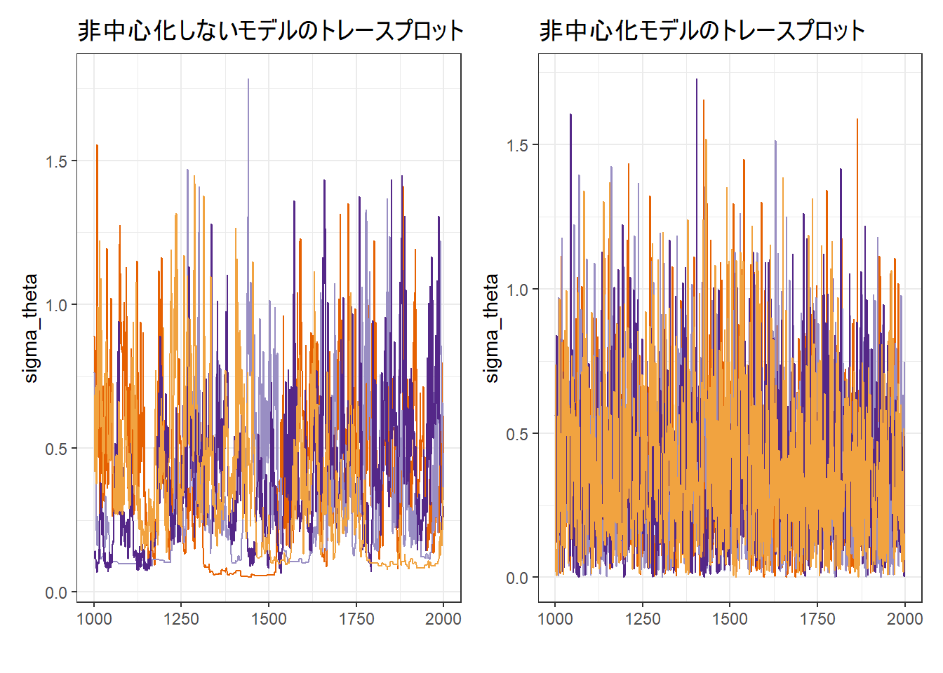
非中心化モデルも決してきれいなトレースプロットではありませんが、非中心化しないモデルよりは改善されていることが確認できます。
結論
本シミュレーション、本サンプルデータにおいては、パラメータを非中心化することで発散的移行をなくし、収束が改善される ことが確認されました。
以上です。