
本ポストはこちらの続きです。

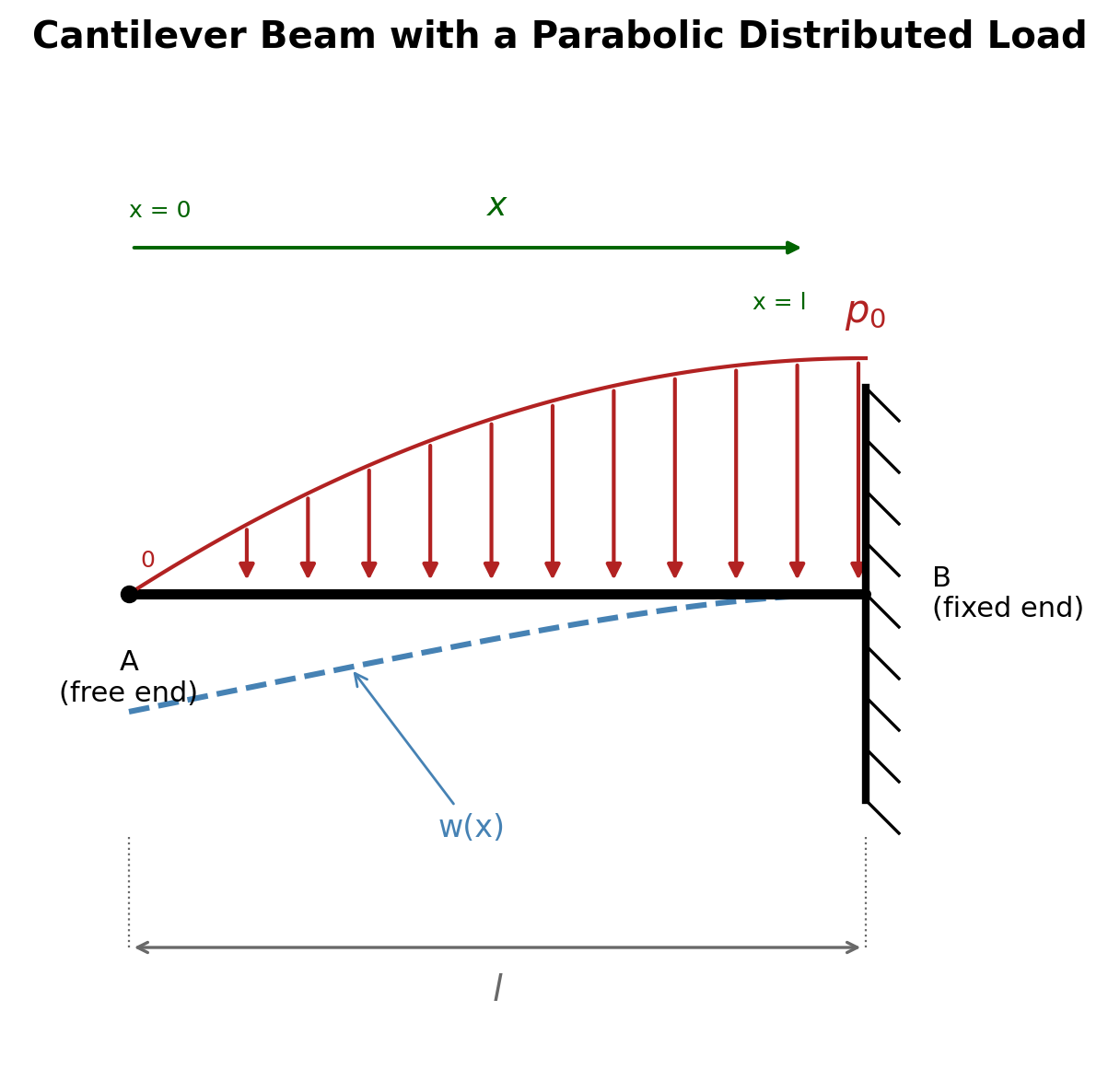
片持ち梁-2次曲線状に変化する分布荷重
片持ち梁のたわみ:FEM(オイラー・ベルヌーイ梁要素) vs 厳密解
ガウス求積の評価点の個数 \(\,n\)、位置 \(\xi_i\) そして重み \(w_i\)につきましては、https://pomax.github.io/bezierinfo/legendre-gauss.html から引用しています。
# ============================================================
# 片持ち梁のたわみ(2次曲線状に変化する分布荷重):FEM vs 厳密解
# ============================================================
#
# 厳密解(xは自由端Aから測った距離):
#   w = -(p0 l^4/360EI){(x/l)^6 - 6(x/l)^5 + 24(x/l) - 19}
#   w_max = (19 p0 l^4)/(360EI)        [x=0, 自由端]
#   θ = (p0 l^3/60EI){(x/l)^5 - 5(x/l)^4 + 4}
#   θ_A = (p0 l^3)/(15EI)
#
#   s : FEM座標(固定端起点、s=0で固定端、s=lで自由端)
#   x : 厳密解の座標(自由端起点、x = l - s)
#
# これまでと同様、荷重をxの関数として素直に定義し、
# ガウス求積による等価節点荷重の計算にそのまま渡す。
# 厳密解が6次式になるため、要素内部にはわずかな誤差が生じる
# (節点上では、これまでと同様に厳密解と一致する)。

library(ggplot2)

# ------------------------------------------------------------
# 1. 梁の諸元と荷重の設定
# ------------------------------------------------------------
l <- 2.0
p0 <- 600 # x=lでの荷重強さ(自由端ではゼロ)[N/m]
E <- 210e9
I <- 4.1667e-6
EI <- E * I

# 分布荷重をxの関数として定義(自由端起点)
q_of_x <- function(x) p0 * (x / l) * (2 - x / l)
q_dist <- function(s) q_of_x(l - s) # FEM座標s(固定端起点)の関数に変換

# ------------------------------------------------------------
# 2. 形状関数と要素剛性行列
# ------------------------------------------------------------
shape_N <- function(xi, Le) {
  N1 <- 1 - 3 * xi^2 + 2 * xi^3
  N2 <- Le * (xi - 2 * xi^2 + xi^3)
  N3 <- 3 * xi^2 - 2 * xi^3
  N4 <- Le * (-xi^2 + xi^3)
  c(N1, N2, N3, N4)
}

beam_element_k <- function(Le) {
  (EI / Le^3) * matrix(c(
    12, 6 * Le, -12, 6 * Le,
    6 * Le, 4 * Le^2, -6 * Le, 2 * Le^2,
    -12, -6 * Le, 12, -6 * Le,
    6 * Le, 2 * Le^2, -6 * Le, 4 * Le^2
  ), nrow = 4, byrow = TRUE)
}

# ------------------------------------------------------------
# 3. 等価節点荷重をガウス求積で数値的に計算する(6点ガウス求積)
# ------------------------------------------------------------
gauss_pts <- c(
  -0.9324695142031521, -0.6612093864662645, -0.2386191860831969,
  0.2386191860831969, 0.6612093864662645, 0.9324695142031521
)
gauss_wts <- c(
  0.1713244923791704, 0.3607615730481386, 0.4679139345726910,
  0.4679139345726910, 0.3607615730481386, 0.1713244923791704
)

beam_element_f <- function(s0, Le) {
  f_e <- numeric(4)
  for (k in seq_along(gauss_pts)) {
    xi <- (gauss_pts[k] + 1) / 2
    jac <- Le / 2
    s <- s0 + xi * Le
    q <- q_dist(s)
    f_e <- f_e + shape_N(xi, Le) * q * jac * gauss_wts[k]
  }
  f_e
}

# ------------------------------------------------------------
# 4. メッシュ生成と全体行列への組み込み
# ------------------------------------------------------------
n_elem <- 10L
Le <- l / n_elem
n_node <- n_elem + 1L
n_dof <- 2L * n_node

K <- matrix(0, n_dof, n_dof)
F <- numeric(n_dof)
K_e <- beam_element_k(Le)

for (e in seq_len(n_elem)) {
  s0 <- (e - 1) * Le
  f_e <- beam_element_f(s0, Le)
  dofs <- c(2 * e - 1, 2 * e, 2 * e + 1, 2 * e + 2)
  K[dofs, dofs] <- K[dofs, dofs] + K_e
  F[dofs] <- F[dofs] + f_e
}

# ------------------------------------------------------------
# 5. 境界条件(固定端: w=0, θ=0)
# ------------------------------------------------------------
fixed_dofs <- c(1, 2)
free_dofs <- setdiff(seq_len(n_dof), fixed_dofs)

u <- numeric(n_dof)
u[free_dofs] <- solve(K[free_dofs, free_dofs], F[free_dofs])

w_fem <- u[seq(1, n_dof, by = 2)]
th_fem <- u[seq(2, n_dof, by = 2)]

s_nodes <- seq(0, l, length.out = n_node)
x_nodes <- l - s_nodes

# ------------------------------------------------------------
# 6. 厳密解との比較
# ------------------------------------------------------------
w_exact_fn <- function(x) {
  xl <- x / l
  -(p0 * l^4) / (360 * EI) * (xl^6 - 6 * xl^5 + 24 * xl - 19)
}

comparison <- data.frame(
  自由端起点_x_m = round(x_nodes, 3),
  FEM近似解_mm = round(w_fem * 1000, 8),
  厳密解_mm = round(w_exact_fn(x_nodes) * 1000, 8),
  差_mm = w_fem * 1000 - w_exact_fn(x_nodes) * 1000
)
print(comparison)

cat("\n自由端でのたわみ量:\n")
cat("  FEM近似解:", w_fem[n_node] * 1000, "mm\n")
cat("  厳密解    :", (19 * p0 * l^4) / (360 * EI) * 1000, "mm\n")

# ------------------------------------------------------------
# 7. 可視化
# ------------------------------------------------------------
hermite_w <- function(xi, Le, w1, th1, w2, th2) {
  N1 <- 1 - 3 * xi^2 + 2 * xi^3
  N2 <- Le * (xi - 2 * xi^2 + xi^3)
  N3 <- 3 * xi^2 - 2 * xi^3
  N4 <- Le * (-xi^2 + xi^3)
  N1 * w1 + N2 * th1 + N3 * w2 + N4 * th2
}

fem_curve <- do.call(rbind, lapply(seq_len(n_elem), function(e) {
  xi_seq <- seq(0, 1, length.out = 20)
  w1v <- w_fem[e]
  th1v <- th_fem[e]
  w2v <- w_fem[e + 1]
  th2v <- th_fem[e + 1]
  s_local <- s_nodes[e] + xi_seq * Le
  data.frame(x = l - s_local, w_mm = hermite_w(xi_seq, Le, w1v, th1v, w2v, th2v) * 1000)
}))

x_fine <- seq(0, l, length.out = 300)
exact_curve <- data.frame(x = x_fine, w_mm = w_exact_fn(x_fine) * 1000)

p1 <- ggplot() +
  geom_line(data = exact_curve, aes(x = x, y = w_mm, color = "厳密解"), linewidth = 1.2) +
  geom_line(
    data = fem_curve, aes(x = x, y = w_mm, color = "FEM(要素内補間)"),
    linetype = "dashed", linewidth = 0.8
  ) +
  geom_point(
    data = data.frame(x = x_nodes, w_mm = w_fem * 1000),
    aes(x = x, y = w_mm, color = "FEM(節点)"), size = 2
  ) +
  scale_color_manual(values = c(
    "厳密解" = "gray40", "FEM(要素内補間)" = "steelblue",
    "FEM(節点)" = "firebrick"
  ), name = "") +
  labs(
    title = "2次曲線状の分布荷重を受ける片持ち梁:FEM vs 厳密解",
    subtitle = paste0("要素数 = ", n_elem, "(節点では一致、要素内部にわずかな差)"),
    x = "自由端からの距離 x [m]", y = "たわみ量 w [mm]"
  ) +
  theme_minimal(base_size = 12)

print(p1)
自由端起点_x_m FEM近似解_mm 厳密解_mm 差_mm
1 2.0 0.00000000 0.00000000 0.000000e+00
2 1.8 0.01254082 0.01254082 -2.853620e-15
3 1.6 0.04583387 0.04583387 -1.112999e-14
4 1.4 0.09419417 0.09419417 -2.486900e-14
5 1.2 0.15298633 0.15298633 -4.093947e-14
6 1.0 0.21856968 0.21856968 -5.681566e-14
7 0.8 0.28822151 0.28822151 -7.238654e-14
8 0.6 0.36003829 0.36003829 -8.792966e-14
9 0.4 0.43281501 0.43281501 -1.040279e-13
10 0.2 0.50590251 0.50590251 -1.206812e-13
11 0.0 0.57904299 0.57904299 -1.375566e-13
自由端でのたわみ量:
FEM近似解: 0.579043 mm
厳密解 : 0.579043 mm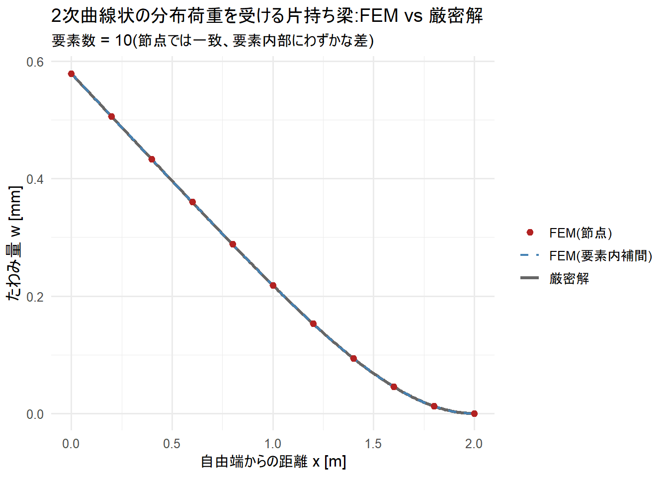
- 荷重 \(p=p_0(x/l)(2-x/l)\) は、自由端Aでゼロ、固定端Bで最大 \(p_0\) となる、放物線状(上に凸)に変化する分布荷重です。
- 節点でのたわみは厳密解と一致し、要素内部の誤差は最大でも0.05μm程度(固定端側で大きく、自由端側で小さい)というごく小さいものでした。
厳密解の公式
- 出典 : 「構造力学公式集 昭和61年版」(土木学会)
荷重・反力・せん断力
\[\begin{eqnarray}p &=& p_0\frac{x}{l}\left(2-\frac{x}{l}\right)\\R_B &=& \frac{2p_0l}{3}\\M_B &=& -\frac{p_0l^2}{4}\\Q &=& \frac{p_0l}{3}\left\{\left(\frac{x}{l}\right)^3-3\left(\frac{x}{l}\right)^2\right\}\end{eqnarray}\]
曲げモーメント
\[\begin{eqnarray}
M &=& \frac{p_0l^2}{12}\left\{\left(\frac{x}{l}\right)^4-4\left(\frac{x}{l}\right)^3\right\}\\
M_{\max} &=& -\frac{p_0l^2}{4}, \quad [x=l]
\end{eqnarray}\]
たわみ
\[\begin{eqnarray}
w &=& -\frac{p_0l^4}{360EI}\left\{\left(\frac{x}{l}\right)^6-6\left(\frac{x}{l}\right)^5+24\left(\frac{x}{l}\right)-19\right\}\\
w_{\max} &=& \frac{19p_0l^4}{360EI}, \quad [x=0]
\end{eqnarray}\]
たわみ角
\[\begin{eqnarray}
\theta &=& \frac{p_0l^3}{60EI}\left\{\left(\frac{x}{l}\right)^5-5\left(\frac{x}{l}\right)^4+4\right\}\\
\theta_A &=& \frac{p_0l^3}{15EI}
\end{eqnarray}\]
以上です。