本ポストは、こちらの続きです。

Rの関数loessの出力 one.delta、two.delta、trace.hatおよびenpをスクラッチで算出
const typesetMath = (el) => { if (window.MathJax) { // MathJax Typeset window.MathJax.typeset(); } else if (window.katex...
www.saecanet.com
2026.06.11
Rの関数 stats::loess により算出される 平滑化曲線(LOESS曲線) をスクラッチで求めます。
処理の流れ
- 自作関数
build_hat_matrixを利用して平滑化行列 / Smoothing Matrix(\(L\)) を求める。 - 観測値 \(y\) と求めた \(L\) から予測値 \(\hat{y}\)(
平滑化曲線 / LOESS曲線) を算出。 \[\hat{\mathbf{y}} = L\mathbf{y}\]
平滑化行列 / Smoothing Matrix 算出のための自作関数
コードを上記ポストから引用します。
build_hat_matrix <- function(x, weights = NULL, span = 0.75, degree = 2L) {
  x <- as.matrix(x)
  N <- nrow(x)
  if (is.null(weights)) weights <- rep(1.0, N)
  # 近傍点数 nf の計算
  nf <- min(N, as.integer(floor(N * span + 1e-5)))
  L <- matrix(0.0, N, N)
  for (j in seq_len(N)) {
    q <- x[j, , drop = TRUE]
    # 二乗距離の計算
    dist2 <- rowSums(sweep(x, 2, q, "-")^2)
    # 近傍 nf 点の選択(partial sort)
    psi <- order(dist2)[seq_len(nf)]
    # バンド幅 rho = nf 番目二乗距離 × max(1, span)
    rho <- dist2[psi[nf]] * max(1.0, span)
    if (rho == 0) rho <- .Machine$double.eps
    # tricube カーネル重みの計算(ehg127 の 2 ループを忠実に再現)
    u <- sqrt(dist2[psi] / rho) # u_i = dist_i / sqrt(rho)
    w_kern <- sqrt(weights[psi] * pmax(0, 1 - u^3)^3) # sqrt(rw * tricube)
    # 重み付きデザイン行列 B = W^{1/2} X (nf × p) の構築
    dx <- x[psi, 1, drop = TRUE] - q[1]
    X_raw <- if (degree == 1L) cbind(1, dx) else cbind(1, dx, dx^2)
    B <- X_raw * w_kern # 各行 i に w_kern[i] を乗算
    # WLS による hat matrix 行 j の計算
    # B^T B = X^T W X  (W = diag(w_kern^2))
    BtB <- crossprod(B)
    BtB_inv <- tryCatch(
      solve(BtB),
      error = function(e) {
        # ランク落ち時は Moore-Penrose 疑似逆行列
        s <- svd(BtB)
        tol <- max(dim(BtB)) * .Machine$double.eps * max(s$d)
        s$v %*% diag(ifelse(s$d > tol, 1 / s$d, 0), length(s$d)) %*% t(s$u)
      }
    )
    # 評価点 j は psi の中で距離 0 の点(必ず含まれる)
    j_idx <- which(psi == j)
    xj <- matrix(X_raw[j_idx, ], nrow = 1) # 1 × p
    # L[j, psi] = xj %*% (X^T W X)^{-1} X^T W
    #           = xj %*% BtB_inv %*% t(B) * w_kern
    # t(B) * w_kern は各列 i に w_kern[i] を乗算 → X^T W に等しい
    L[j, psi] <- as.numeric(xj %*% BtB_inv %*% t(B) * w_kern)
  }
  L
}
サンプルデータの生成
seed <- 20260613
set.seed(seed)
n <- 50
x <- seq(0, 2 * pi, length.out = n)
y <- sin(x) + rnorm(n, 0, 0.2)
w <- rep(1, n)
平滑化行列 / Smoothing Matrix(hat matrix) L の構築と予測値の計算
L <- build_hat_matrix(x, weights = w, span = 0.75, degree = 2L)
y_hat <- as.numeric(L %*% y) # 予測値: ŷ = L y

cat("--- 平滑化行列 / Smoothing Matrix の一部を確認 ---\n")
str(L)
--- 平滑化行列 / Smoothing Matrix の一部を確認 ---
num [1:50, 1:50] 0.284 0.242 0.203 0.168 0.135 ... stats::loess による予測値の算出
fit <- loess(y ~ x,
  span = 0.75, degree = 2, weights = w,
  control = loess.control(
    surface = "direct",
    statistics = "exact",
    trace.hat = "exact"
  )
)
y_hat_ref <- fitted(fit)自作関数build_hat_matrixと関数stats::loessの比較
library(ggplot2)

# ------------------------------------------------------------
# プロット用データフレーム
# ------------------------------------------------------------
df <- data.frame(
  x         = x,
  y_obs     = y, # 観測値
  y_scratch = y_hat, # 自作関数予測値 (L %*% y)
  y_loess   = y_hat_ref # 関数loess の予測値(参照)
)

# ------------------------------------------------------------
# ggplot によるプロット
# ------------------------------------------------------------
p <- ggplot(df, aes(x = x)) +

  # 観測値(散布図)
  geom_point(aes(y = y_obs, colour = "観測値"),
    size = 2, alpha = 0.7
  ) +

  # 自作関数予測値 L %*% y(実線)
  geom_line(aes(y = y_scratch, colour = "自作関数  (L %*% y)"),
    linewidth = 1.0
  ) +

  # 関数loess 予測値(破線)
  geom_line(aes(y = y_loess, colour = "関数loess fitted"),
    linewidth = 1.6, linetype = "dashed"
  ) +

  # 凡例・軸ラベル
  scale_colour_manual(
    name = NULL,
    values = c(
      "観測値" = "#888888",
      "自作関数  (L %*% y)" = "#2166AC",
      "関数loess fitted" = "#D6604D"
    ),
    breaks = c("観測値", "自作関数  (L %*% y)", "関数loess fitted")
  ) +
  labs(
    title    = expression(paste("loess  ", hat(bold(y)), " = ", bold(L), bold(y))),
    subtitle = "span = 0.75,  degree = 2,  n = 50",
    x        = "x",
    y        = "y"
  ) +
  theme_bw(base_size = 13) +
  theme(
    legend.position  = "bottom",
    plot.title       = element_text(face = "bold"),
    panel.grid.minor = element_blank()
  )

print(p)

cat(paste0("両関数の結果は一致しているか: ", all.equal(y_hat, y_hat_ref)))
両関数の結果は一致しているか: TRUE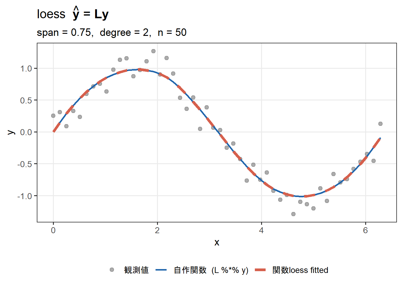
以上です。