
本ポストはこちらの続きです。

Rで有限要素法:片持ち梁-2次曲線状に凸型で変化する分布荷重:たわみ量
const typesetMath = (el) => { if (window.MathJax) { // MathJax Typeset window.MathJax.typeset(); } else if (window.katex...
www.saecanet.com
2026.09.27
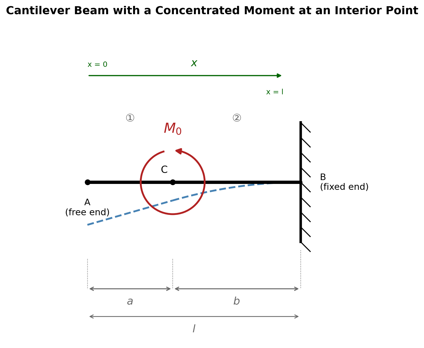
片持ち梁-中間点に集中モーメント
片持ち梁のたわみ:FEM(オイラー・ベルヌーイ梁要素) vs 厳密解
# ============================================================
# 片持ち梁のたわみ(中間点に集中モーメント):FEM vs 厳密解
# ============================================================
#
# 厳密解(xは自由端Aから測った距離):
#   w1 = (M0 l/2EI){2x(α-1) + l(1-α^2)}             [0<=x<=a]
#   w2 = (M0 l^2/2EI){(x/l)^2 - 2(x/l) + 1}          [a<=x<=l]
#   w_max = (M0 l^2/2EI)(1-α^2)                      [x=0, 自由端]
#
#   s : FEM座標(固定端起点、s=0で固定端、s=lで自由端)
#   x : 厳密解の座標(自由端起点、x = l - s)
#
# 集中モーメントの等価節点荷重:
#   モーメントがする仕事は「モーメント×回転角」であり、回転角はdw/ds。
#   荷重点での形状関数の傾き dN_i/ds を使って、f_e = M * dN_i/ds とする。
#   荷重点が節点上にあれば、その節点の傾き自由度に直接M0を与えるのと同じになる。
#
# 符号について:
#   厳密解ではM2=-M0で、たわみは下向き(正)になる。
#   FEMのs方向の傾き自由度には、+M0を与えると厳密解と一致する。

library(ggplot2)

# ------------------------------------------------------------
# 1. 梁の諸元と荷重の設定
# ------------------------------------------------------------
l <- 2.0
a <- 0.8 # 自由端Aから点Cまでの距離
b <- l - a # 点Cから固定端Bまでの距離
alpha <- a / l
M0 <- 2000 # 点Cに作用する集中モーメント [N・m]
E <- 210e9
I <- 4.1667e-6
EI <- E * I

s_load <- l - a # 点CのFEM座標(固定端起点)

# ------------------------------------------------------------
# 2. 形状関数、その傾き、要素剛性行列
# ------------------------------------------------------------
# 傾きは、要素内座標xiでの微分を要素長Leで割って、s方向の微分に直したもの
shape_dN <- function(xi, Le) {
  c(
    (-6 * xi + 6 * xi^2) / Le,
    1 - 4 * xi + 3 * xi^2,
    (6 * xi - 6 * xi^2) / Le,
    -2 * xi + 3 * xi^2
  )
}

beam_element_k <- function(Le) {
  (EI / Le^3) * matrix(c(
    12, 6 * Le, -12, 6 * Le,
    6 * Le, 4 * Le^2, -6 * Le, 2 * Le^2,
    -12, -6 * Le, 12, -6 * Le,
    6 * Le, 2 * Le^2, -6 * Le, 4 * Le^2
  ), nrow = 4, byrow = TRUE)
}

# ------------------------------------------------------------
# 3. メッシュ生成と全体行列への組み込み
# ------------------------------------------------------------
n_elem <- 10L # Le=0.2、s_load=1.2はその6倍 → 点Cにちょうど節点が来る
Le <- l / n_elem
n_node <- n_elem + 1L
n_dof <- 2L * n_node

K <- matrix(0, n_dof, n_dof)
F <- numeric(n_dof)
K_e <- beam_element_k(Le)

for (e in seq_len(n_elem)) {
  dofs <- c(2 * e - 1, 2 * e, 2 * e + 1, 2 * e + 2)
  K[dofs, dofs] <- K[dofs, dofs] + K_e
}

# ------------------------------------------------------------
# 4. 集中モーメントの載荷(荷重点を含む要素を探し、形状関数の傾きで等価節点荷重に変換)
# ------------------------------------------------------------
# 1e-9は、s_load/Leが整数のとき丸め誤差で隣の要素に振り分けられるのを防ぐための微小量
e_idx <- min(floor(s_load / Le + 1e-9) + 1L, n_elem) # 荷重点を含む要素番号(1始まり)
xi0 <- (s_load - (e_idx - 1) * Le) / Le # 要素内のローカル座標
xi0 <- min(max(xi0, 0), 1) # 丸め誤差で範囲外に出た分を戻す

f_e <- shape_dN(xi0, Le) * M0
dofs <- c(2 * e_idx - 1, 2 * e_idx, 2 * e_idx + 1, 2 * e_idx + 2)
F[dofs] <- F[dofs] + f_e

# ------------------------------------------------------------
# 5. 境界条件(固定端: w=0, θ=0)
# ------------------------------------------------------------
fixed_dofs <- c(1, 2)
free_dofs <- setdiff(seq_len(n_dof), fixed_dofs)

u <- numeric(n_dof)
u[free_dofs] <- solve(K[free_dofs, free_dofs], F[free_dofs])

w_fem <- u[seq(1, n_dof, by = 2)]
th_fem <- u[seq(2, n_dof, by = 2)]

s_nodes <- seq(0, l, length.out = n_node)
x_nodes <- l - s_nodes

# ------------------------------------------------------------
# 6. 厳密解との比較(点Cを境に2つの式を使い分ける)
# ------------------------------------------------------------
w_exact_fn <- function(x) {
  ifelse(x <= a,
    (M0 * l) / (2 * EI) * (2 * x * (alpha - 1) + l * (1 - alpha^2)),
    (M0 * l^2) / (2 * EI) * ((x / l)^2 - 2 * (x / l) + 1)
  )
}

comparison <- data.frame(
  自由端起点_x_m = round(x_nodes, 3),
  FEM近似解_mm = round(w_fem * 1000, 8),
  厳密解_mm = round(w_exact_fn(x_nodes) * 1000, 8),
  差_mm = w_fem * 1000 - w_exact_fn(x_nodes) * 1000
)
print(comparison)

cat("\n自由端でのたわみ量:\n")
cat("  FEM近似解:", w_fem[n_node] * 1000, "mm\n")
cat("  厳密解    :", (M0 * l^2) / (2 * EI) * (1 - alpha^2) * 1000, "mm\n")

# ------------------------------------------------------------
# 7. 可視化
# ------------------------------------------------------------
hermite_w <- function(xi, Le, w1, th1, w2, th2) {
  N1 <- 1 - 3 * xi^2 + 2 * xi^3
  N2 <- Le * (xi - 2 * xi^2 + xi^3)
  N3 <- 3 * xi^2 - 2 * xi^3
  N4 <- Le * (-xi^2 + xi^3)
  N1 * w1 + N2 * th1 + N3 * w2 + N4 * th2
}

fem_curve <- do.call(rbind, lapply(seq_len(n_elem), function(e) {
  xi_seq <- seq(0, 1, length.out = 20)
  w1v <- w_fem[e]
  th1v <- th_fem[e]
  w2v <- w_fem[e + 1]
  th2v <- th_fem[e + 1]
  s_local <- s_nodes[e] + xi_seq * Le
  data.frame(x = l - s_local, w_mm = hermite_w(xi_seq, Le, w1v, th1v, w2v, th2v) * 1000)
}))

x_fine <- seq(0, l, length.out = 300)
exact_curve <- data.frame(x = x_fine, w_mm = w_exact_fn(x_fine) * 1000)

p1 <- ggplot() +
  geom_line(data = exact_curve, aes(x = x, y = w_mm, color = "厳密解"), linewidth = 1.2) +
  geom_line(
    data = fem_curve, aes(x = x, y = w_mm, color = "FEM(要素内補間)"),
    linetype = "dashed", linewidth = 0.8
  ) +
  geom_point(
    data = data.frame(x = x_nodes, w_mm = w_fem * 1000),
    aes(x = x, y = w_mm, color = "FEM(節点)"), size = 2
  ) +
  geom_vline(xintercept = a, linetype = "dotted", color = "gray50") +
  scale_color_manual(values = c(
    "厳密解" = "gray40", "FEM(要素内補間)" = "steelblue",
    "FEM(節点)" = "firebrick"
  ), name = "") +
  labs(
    title = "中間点に集中モーメントを受ける片持ち梁:FEM vs 厳密解",
    subtitle = paste0("要素数 = ", n_elem, "(点線はモーメント作用点C)"),
    x = "自由端からの距離 x [m]", y = "たわみ量 w [mm]"
  ) +
  theme_minimal(base_size = 12)

print(p1)
自由端起点_x_m FEM近似解_mm 厳密解_mm 差_mm
1 2.0 0.00000000 0.00000000 0.000000e+00
2 1.8 0.04571392 0.04571392 -1.674355e-14
3 1.6 0.18285568 0.18285568 -6.658563e-14
4 1.4 0.41142528 0.41142528 -1.473821e-13
5 1.2 0.73142272 0.73142272 -2.471356e-13
6 1.0 1.14284800 1.14284800 -3.563816e-13
7 0.8 1.64570112 1.64570112 -4.722889e-13
8 0.6 2.19426816 2.19426816 -5.879741e-13
9 0.4 2.74283520 2.74283520 -7.012169e-13
10 0.2 3.29140224 3.29140224 -8.126833e-13
11 0.0 3.83996928 3.83996928 -9.277024e-13
自由端でのたわみ量:
FEM近似解: 3.839969 mm
厳密解 : 3.839969 mm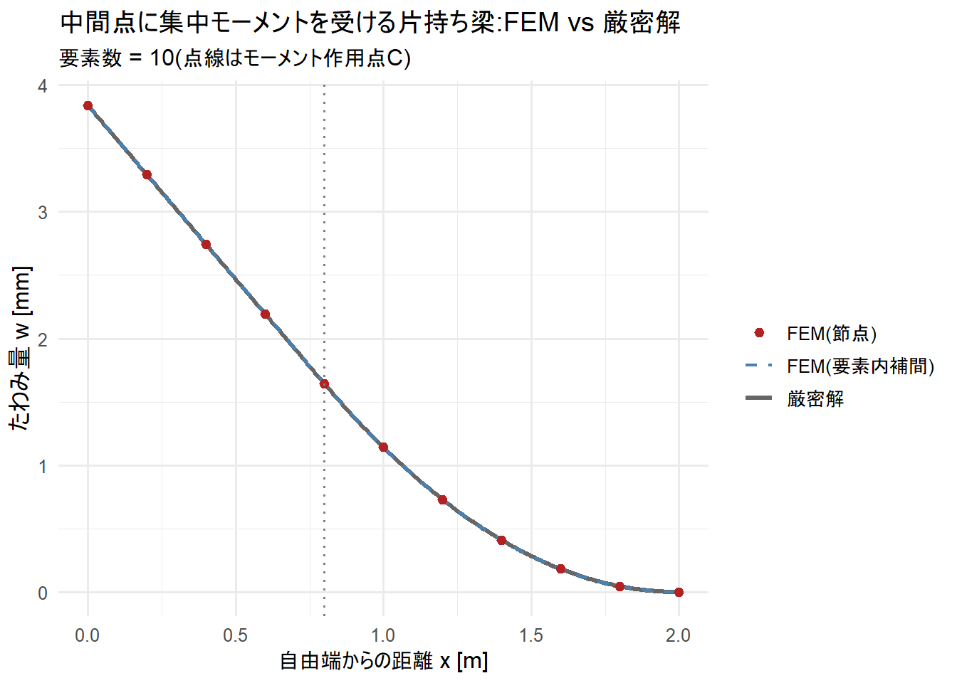
厳密解の公式
- 出典 : 「構造力学公式集 昭和61年版」(土木学会)
反力・せん断力
\[\begin{eqnarray}R_B &=& 0\\M_B &=& -M_0\\Q_1 &=& 0\\Q_2 &=& 0\end{eqnarray}\]
曲げモーメント
\[\begin{eqnarray}
M_1 &=& 0\\
M_2 &=& -M_0\\
M_{\max} &=& -M_0, \quad [x>a]
\end{eqnarray}\]
たわみ
\[\begin{eqnarray}
w_1 &=& \frac{M_0l}{2EI}\left\{2x(\alpha-1)+l(1-\alpha^2)\right\}\\
w_2 &=& \frac{M_0l^2}{2EI}\left\{\left(\frac{x}{l}\right)^2-2\left(\frac{x}{l}\right)+1\right\}\\
w_{\max} &=& \frac{M_0l^2}{2EI}(1-\alpha^2), \quad [x=0]
\end{eqnarray}\]
たわみ角
\[\begin{eqnarray}
\theta_1 &=& \frac{M_0b}{EI}\\
\theta_2 &=& \frac{M_0l}{EI}\left(1-\frac{x}{l}\right)\\
\theta_A &=& \frac{M_0b}{EI}
\end{eqnarray}\]
変数の定義:
- \(M_0\)は点Cに作用する集中モーメント、\(a\)は自由端Aから点Cまでの距離、\(b\)は点Cから固定端Bまでの距離(\(a+b=l\))、\(\alpha=a/l\)、\(x\)は自由端Aから測った距離、区間①は \(0\le x\le a\)、区間②は \(a\le x\le l\) です。
以上です。