本ポストはこちらの続きです。

Rで有限要素法:片持ち梁-全スパン等分布荷重:たわみ量
const typesetMath = (el) => { if (window.MathJax) { // MathJax Typeset window.MathJax.typeset(); } else if (window.katex...
www.saecanet.com
2026.08.31
片持ち梁-三角形状分布荷重
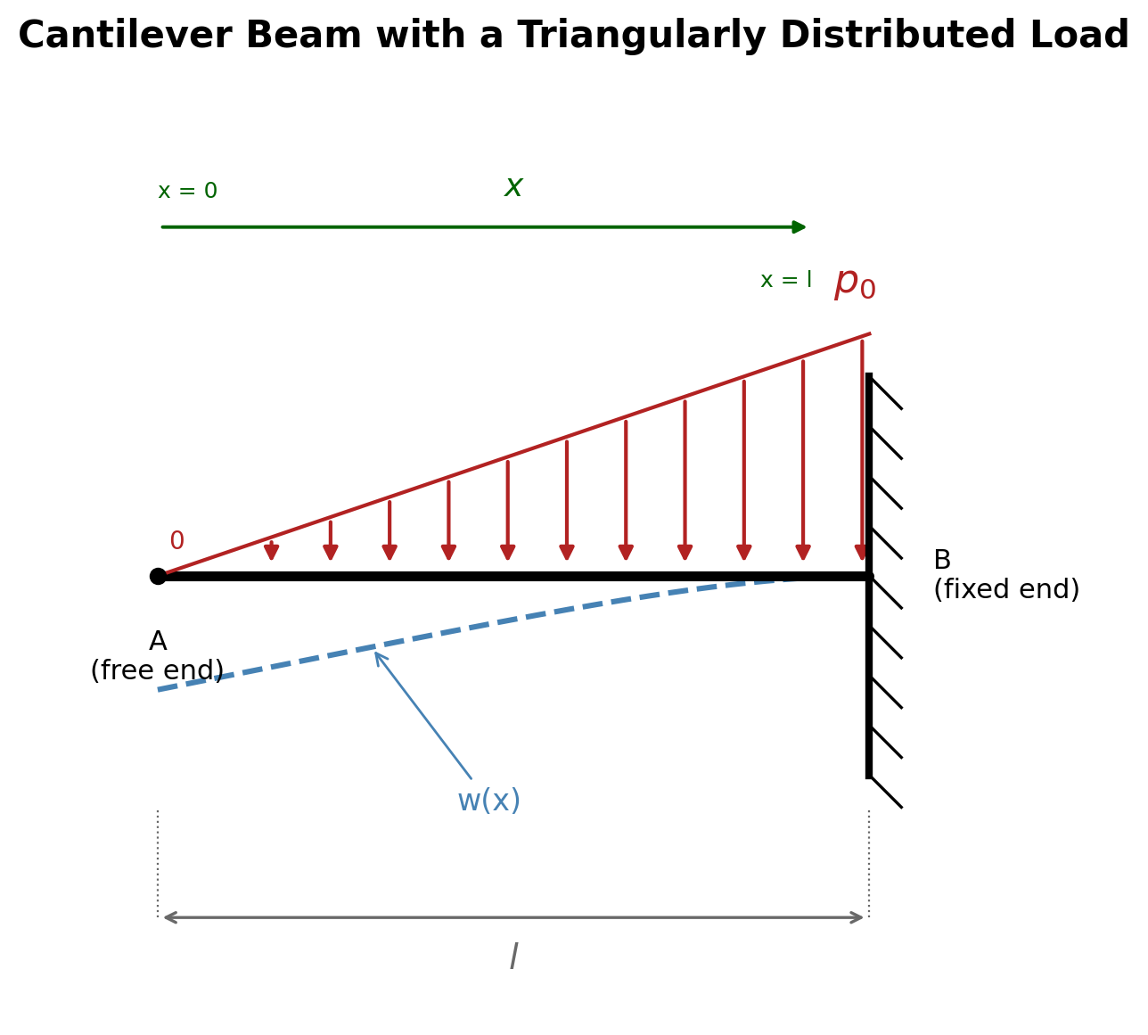
片持ち梁のたわみ:FEM(オイラー・ベルヌーイ梁要素) vs 厳密解
# ============================================================
# 片持ち梁のたわみ(三角形分布荷重):FEM vs 厳密解
# ============================================================
#
# 厳密解(xは自由端Aから測った距離):
#   w(x)  = (p0 l^4)/(120EI) * { 4 - 5(x/l) + (x/l)^5 }
#   w_max = (p0 l^4)/(30EI)          [x = 0, 自由端]
#   θ(x)  = (p0 l^3)/(24EI) * { 1 - (x/l)^4 }
#   θ_A   = (p0 l^3)/(24EI)          [x = 0, 自由端]
#
# 集中荷重、等分布荷重との違い:
#   厳密解が5次式になる(集中荷重は3次式、等分布荷重は4次式)。
#   荷重自体も一定ではなく、位置によって直線的に変化する。
#   このため等価節点荷重は、これまでのような単純な式ではなく、
#   汎用性の高いガウス求積による数値積分で求める。
#
#   s   : FEM座標(固定端起点、s=0で固定端、s=lで自由端)
#   x   : 厳密解の座標(自由端起点、x = l - s)

library(ggplot2)

# ------------------------------------------------------------
# 1. 梁の諸元と荷重の設定
# ------------------------------------------------------------
l <- 2.0
p0 <- 800 # 固定端での荷重強さ [N/m](自由端でゼロ)
E <- 210e9
I <- 4.1667e-6
EI <- E * I

# 分布荷重をFEM座標s(固定端起点)の関数として定義
# s=0(固定端)でp0、s=l(自由端)でゼロとなる直線
q_dist <- function(s) p0 * (1 - s / l)

# ------------------------------------------------------------
# 2. 形状関数と要素剛性行列
# ------------------------------------------------------------
shape_N <- function(xi, Le) {
  N1 <- 1 - 3 * xi^2 + 2 * xi^3
  N2 <- Le * (xi - 2 * xi^2 + xi^3)
  N3 <- 3 * xi^2 - 2 * xi^3
  N4 <- Le * (-xi^2 + xi^3)
  c(N1, N2, N3, N4)
}

beam_element_k <- function(Le) {
  (EI / Le^3) * matrix(c(
    12, 6 * Le, -12, 6 * Le,
    6 * Le, 4 * Le^2, -6 * Le, 2 * Le^2,
    -12, -6 * Le, 12, -6 * Le,
    6 * Le, 2 * Le^2, -6 * Le, 4 * Le^2
  ), nrow = 4, byrow = TRUE)
}

# ------------------------------------------------------------
# 3. 等価節点荷重をガウス求積で数値的に計算する
#    (形状関数×荷重を要素内で積分することで、荷重を節点に置き換える)
# ------------------------------------------------------------
gauss_pts <- c(
  -sqrt((3 - 2 * sqrt(6 / 5)) / 7), -sqrt((3 + 2 * sqrt(6 / 5)) / 7),
  sqrt((3 - 2 * sqrt(6 / 5)) / 7), sqrt((3 + 2 * sqrt(6 / 5)) / 7)
)
gauss_wts <- c(
  (18 + sqrt(30)) / 36, (18 - sqrt(30)) / 36,
  (18 + sqrt(30)) / 36, (18 - sqrt(30)) / 36
) # 4点ガウス求積(区間[-1,1])

beam_element_f <- function(s0, Le) {
  f_e <- numeric(4)
  for (k in seq_along(gauss_pts)) {
    xi <- (gauss_pts[k] + 1) / 2 # [-1,1] を [0,1] に変換
    jac <- Le / 2
    s <- s0 + xi * Le
    q <- q_dist(s)
    f_e <- f_e + shape_N(xi, Le) * q * jac * gauss_wts[k]
  }
  f_e
}

# ------------------------------------------------------------
# 4. メッシュ生成・全体行列への組み込み
# ------------------------------------------------------------
n_elem <- 8L
Le <- l / n_elem
n_node <- n_elem + 1L
n_dof <- 2L * n_node

K <- matrix(0, n_dof, n_dof)
F <- numeric(n_dof)
K_e <- beam_element_k(Le) # 等間隔分割のため要素剛性行列は共通

for (e in seq_len(n_elem)) {
  s0 <- (e - 1) * Le
  f_e <- beam_element_f(s0, Le)
  dofs <- c(2 * e - 1, 2 * e, 2 * e + 1, 2 * e + 2)
  K[dofs, dofs] <- K[dofs, dofs] + K_e
  F[dofs] <- F[dofs] + f_e
}

# ------------------------------------------------------------
# 5. 境界条件(固定端: w=0, θ=0)
# ------------------------------------------------------------
fixed_dofs <- c(1, 2)
free_dofs <- setdiff(seq_len(n_dof), fixed_dofs)

u <- numeric(n_dof)
u[free_dofs] <- solve(K[free_dofs, free_dofs], F[free_dofs])

w_fem <- u[seq(1, n_dof, by = 2)]
th_fem <- u[seq(2, n_dof, by = 2)]

s_nodes <- seq(0, l, length.out = n_node)
x_nodes <- l - s_nodes

# ------------------------------------------------------------
# 6. 厳密解との比較
# ------------------------------------------------------------
w_exact_fn <- function(x) (p0 * l^4) / (120 * EI) * (4 - 5 * (x / l) + (x / l)^5)

comparison <- data.frame(
  自由端起点_x_m = round(x_nodes, 3),
  FEM近似解_mm = round(w_fem * 1000, 8),
  厳密解_mm = round(w_exact_fn(x_nodes) * 1000, 8),
  差_mm = w_fem * 1000 - w_exact_fn(x_nodes) * 1000
)
print(comparison)

cat("\n自由端でのたわみ量:\n")
cat("  FEM近似解:", w_fem[n_node] * 1000, "mm\n")
cat("  厳密解    :", p0 * l^4 / (30 * EI) * 1000, "mm  (公式: w_max = p0 l^4 / 30EI)\n")

# ------------------------------------------------------------
# 7. 要素内部を含めた可視化と誤差の確認
# ------------------------------------------------------------
hermite_w <- function(xi, Le, w1, th1, w2, th2) {
  N1 <- 1 - 3 * xi^2 + 2 * xi^3
  N2 <- Le * (xi - 2 * xi^2 + xi^3)
  N3 <- 3 * xi^2 - 2 * xi^3
  N4 <- Le * (-xi^2 + xi^3)
  N1 * w1 + N2 * th1 + N3 * w2 + N4 * th2
}

fem_curve <- do.call(rbind, lapply(seq_len(n_elem), function(e) {
  xi_seq <- seq(0, 1, length.out = 20)
  w1 <- w_fem[e]
  th1 <- th_fem[e]
  w2 <- w_fem[e + 1]
  th2 <- th_fem[e + 1]
  s_local <- s_nodes[e] + xi_seq * Le
  data.frame(x = l - s_local, w_mm = hermite_w(xi_seq, Le, w1, th1, w2, th2) * 1000)
}))
fem_curve$w_exact_mm <- w_exact_fn(fem_curve$x) * 1000
fem_curve$diff_um <- (fem_curve$w_mm - fem_curve$w_exact_mm) * 1000

x_fine <- seq(0, l, length.out = 300)
exact_curve <- data.frame(x = x_fine, w_mm = w_exact_fn(x_fine) * 1000)

p1 <- ggplot() +
  geom_line(data = exact_curve, aes(x = x, y = w_mm, color = "厳密解"), linewidth = 1.2) +
  geom_line(
    data = fem_curve, aes(x = x, y = w_mm, color = "FEM(要素内補間)"),
    linetype = "dashed", linewidth = 0.8
  ) +
  geom_point(
    data = data.frame(x = x_nodes, w_mm = w_fem * 1000),
    aes(x = x, y = w_mm, color = "FEM(節点)"), size = 2
  ) +
  scale_color_manual(values = c(
    "厳密解" = "gray40", "FEM(要素内補間)" = "steelblue",
    "FEM(節点)" = "firebrick"
  ), name = "") +
  labs(
    title = "三角形分布荷重を受ける片持ち梁のたわみ曲線:FEM vs 厳密解",
    subtitle = paste0("要素数 = ", n_elem, "(節点では一致、要素内部にわずかな差)"),
    x = "自由端からの距離 x [m]", y = "たわみ量 w [mm]"
  ) +
  theme_minimal(base_size = 12)

p2 <- ggplot(fem_curve, aes(x = x, y = diff_um)) +
  geom_line(color = "darkred") +
  geom_hline(yintercept = 0, linetype = "dotted") +
  labs(
    title = "要素内部での誤差(FEM補間 - 厳密解)",
    subtitle = "荷重が大きい固定端側(x大)で誤差も大きくなる",
    x = "自由端からの距離 x [m]", y = "差 [μm]"
  ) +
  theme_minimal(base_size = 12)

print(p1)
print(p2)
自由端起点_x_m FEM近似解_mm 厳密解_mm 差_mm
1 2.00 0.00000000 0.00000000 0.000000e+00
2 1.75 0.01681162 0.01681162 2.702699e-15
3 1.50 0.05940429 0.05940429 1.021405e-14
4 1.25 0.11829146 0.11829146 2.159384e-14
5 1.00 0.18666517 0.18666517 3.572143e-14
6 0.75 0.25994956 0.25994956 5.156986e-14
7 0.50 0.33535446 0.33535446 6.861178e-14
8 0.25 0.41142900 0.41142900 8.637535e-14
9 0.00 0.48761515 0.48761515 1.045275e-13
自由端でのたわみ量:
FEM近似解: 0.4876151 mm
厳密解 : 0.4876151 mm (公式: w_max = p0 l^4 / 30EI)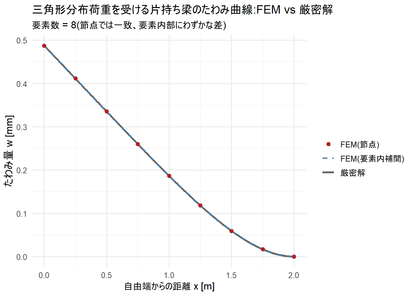
荷重が一定ではなく直線的に変化するため、等価節点荷重を単純な式で書き下すのではなく、4点ガウス求積による数値積分で計算しています。
これにより、荷重の与え方(一定・直線・その他の分布)が変わっても関数 beam_element_f を書き換えるだけで対応できる、汎用的な作りになっています。
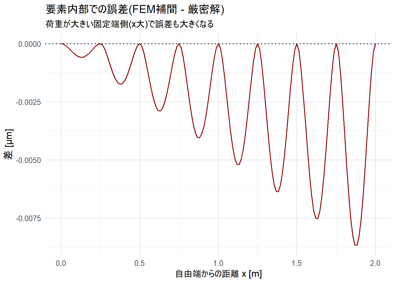
節点でのたわみは厳密解と完全に一致し、要素内部の誤差は固定端に近いほど大きく(荷重が大きいほど誤差も大きい)、自由端に近いほど小さくなる、という結果でした。
厳密解が5次式になったことで、等分布荷重(4次式・誤差が要素ごとに一定)とは異なる誤差の分布になっています。
以上です。